
Technology
What makes
seeing possible.
Our technology has two sides: the sensor and the decision. The sensor measures the direction a surface faces, assembles that into height, and captures one row at a time even on a line that never stops. The engine counts the distance from good products and notices the difference. This page describes those methods themselves, separately from any product name.
It exists to answer, in advance, the questions we are always asked across a table.
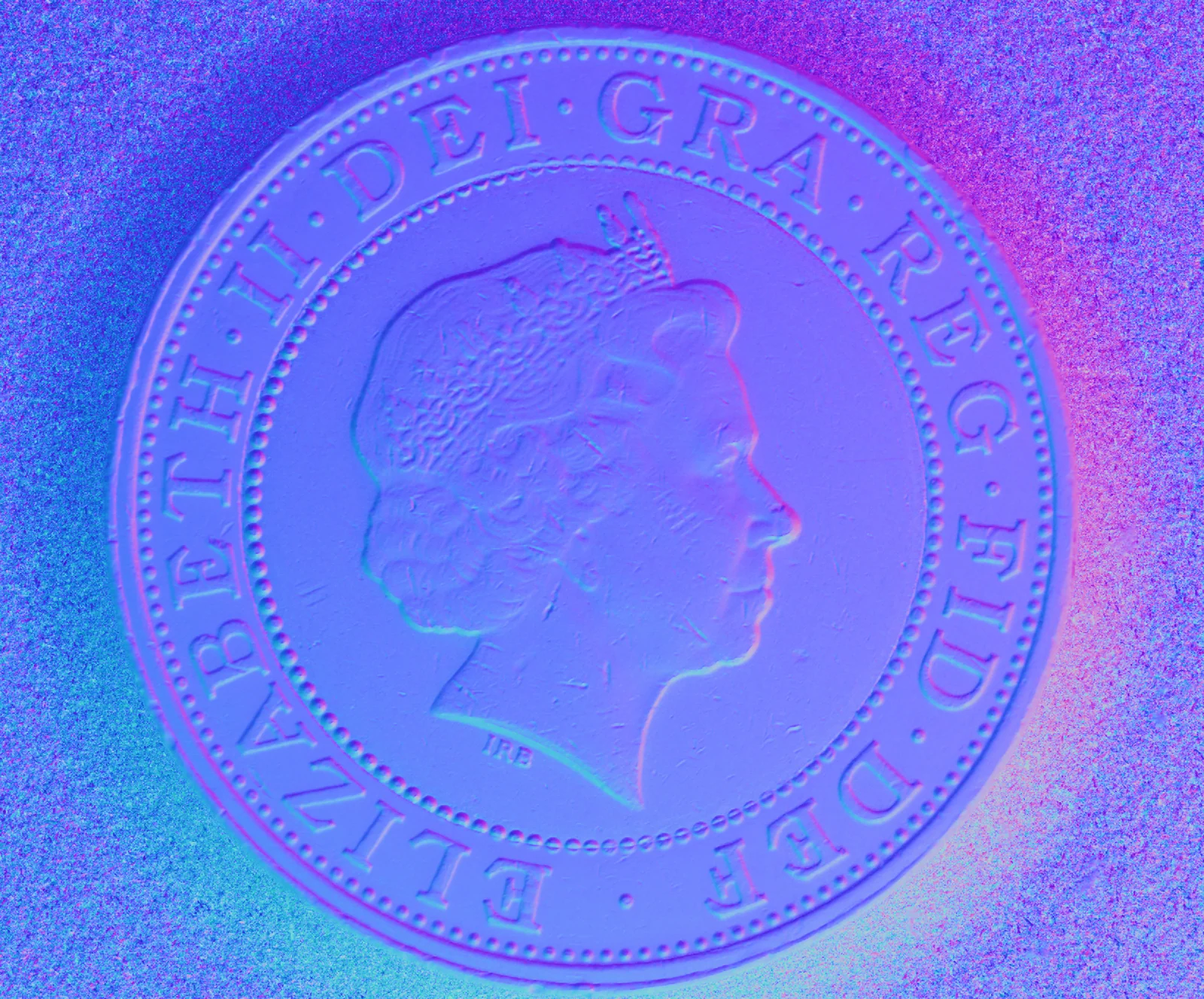
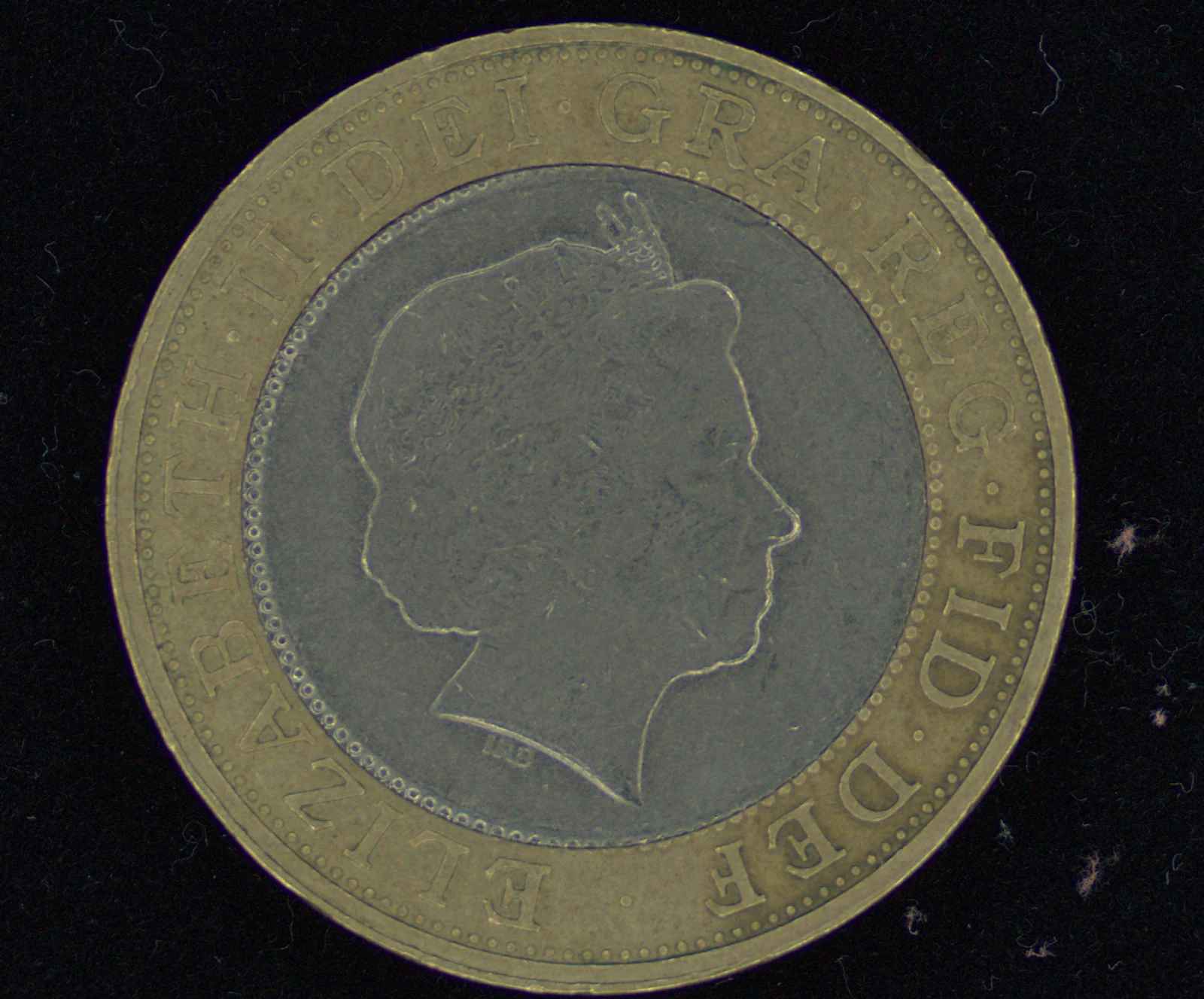
◀ Drag to compare ▶
The surface normal taken from a single capture. Everything this site claims begins here.
Explainers
Seven methods, in outline.
Not product specifications: the principle, and the limits. Each page puts hands-on experiments first, so it starts from doing rather than from claims. More explainers will follow.
Capturing — what the sensor measures
Move the light, and measure the direction a surface faces. What separates it from triangulation-based 3D, whether the result holds when the lighting changes, and how few images are enough.
Try it — move the light / how many images solve it
Read the explainer →

Assemble height out of surface direction. Why adding from one edge leaves streaks, where the error accumulates, and whether height can be read in micrometres.
Try it — integrate and rotate / where the error builds up
Read the explainer →
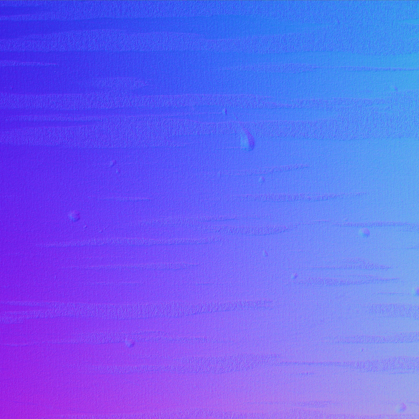
Using photometric stereo on something in motion, with a camera that takes one row at a time. What decides the vertical size of the image, whether an encoder is needed, how the lighting switch is synchronised, and how much data flows.
Try it — capture one row at a time / switch the lighting as it flows / work out the data rate
Read the explainer →
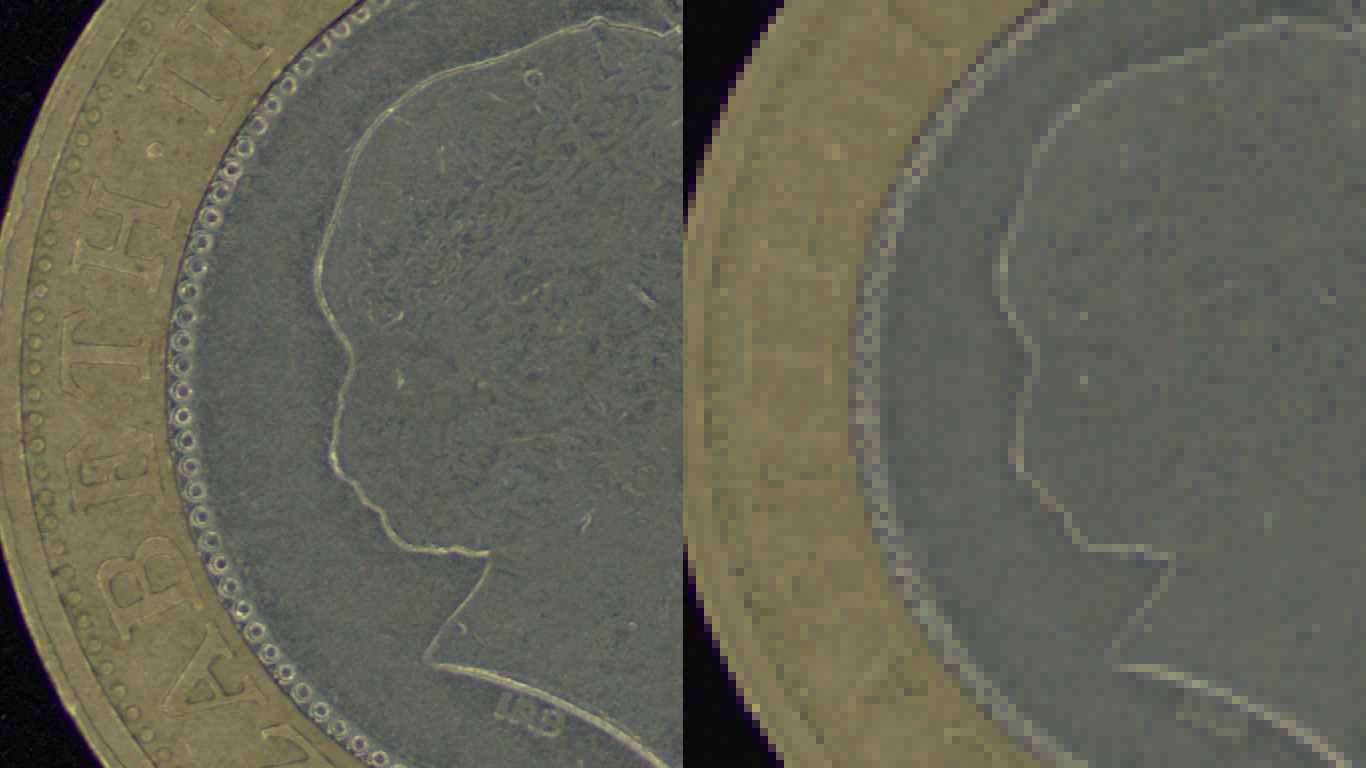
How small a flaw can be seen. The real size of one pixel, which is field of view divided by pixel count, and how many pixels a thing needs before it can be called visible.
Try it — place one pixel on the real object / where dots stop being dots
Read the explainer →
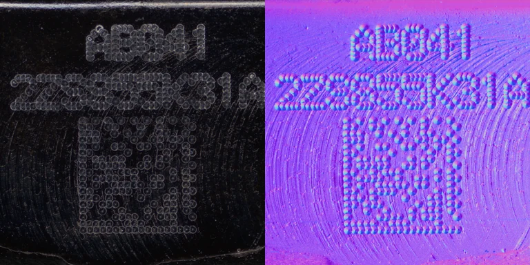
How black plastic, plated faces, transparent coatings and fine relief each come out. Six materials measured, so the difference between the photograph and the surface direction can be read directly.
Try it — the photo line and the direction line / where the six fall
Read the explainer →
Deciding — what the engine counts
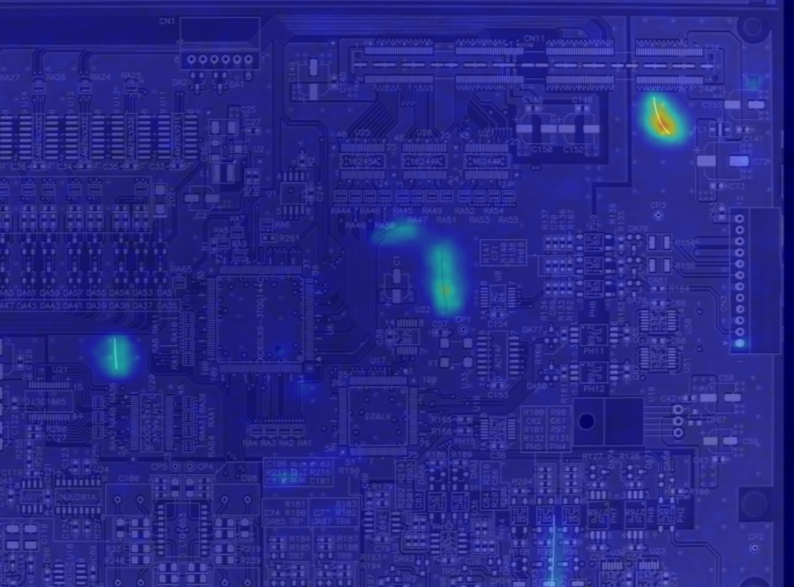
Learn good products only, and notice the difference. Whether a verdict is really possible without collecting defects, who sets the threshold, and what Human_Check is.
Try it — make it remember good products / place the thresholds
Read the explainer →
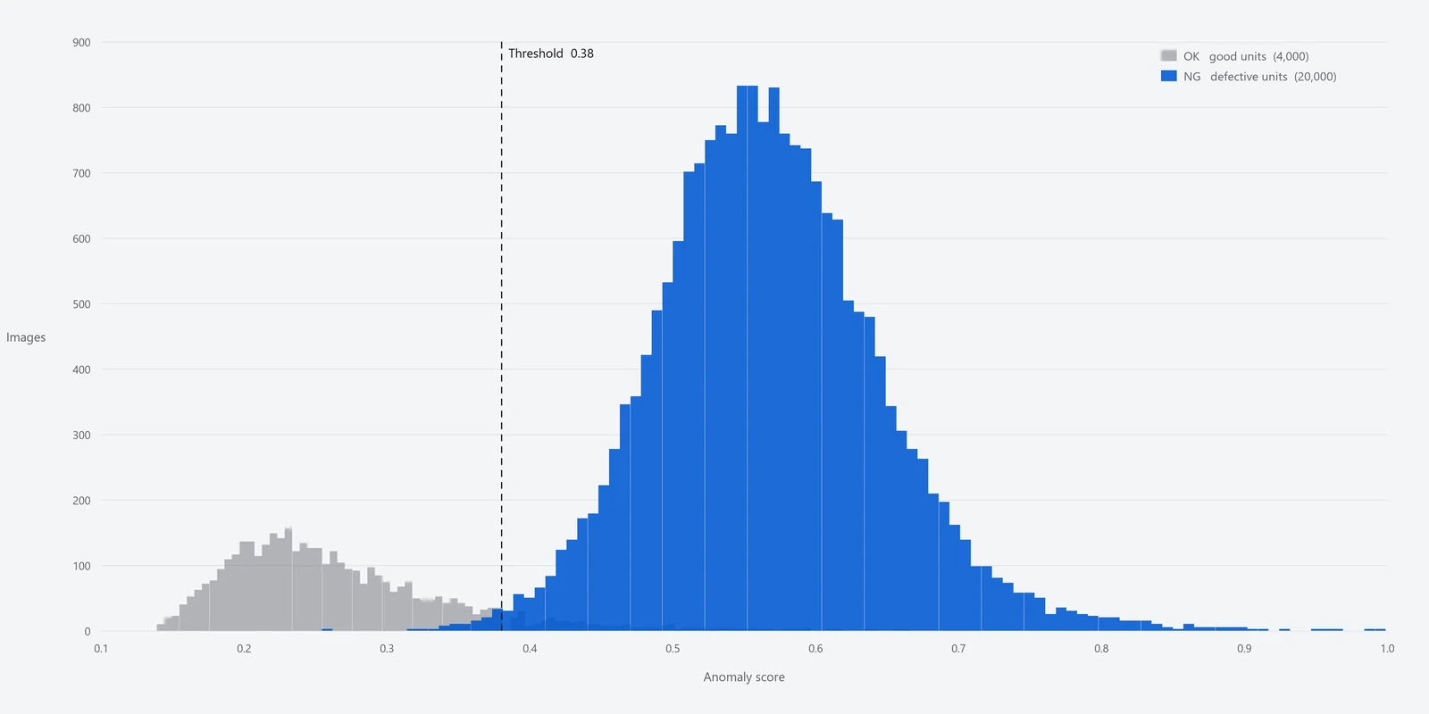
Why “what is the accuracy?” has no single-number answer. The trade-off between misses and false alarms, precision that moves with the defect rate on your line, and sample size against confidence.
Try it — run 10,000 pieces through / how many was that number measured on
Read the explainer →
※ On the Japanese site each of these methods has its own page, with blocks you can operate in the browser to check the claim for yourself. English versions of those explainer pages are 〔要確認〕. The questions below carry the same short answers.
Frequently asked
The questions we are asked,
with short answers.
These are the questions put to us across a table, kept as they are asked.
On capturing — photometric stereo
| Question | Short answer | Where to check |
|---|---|---|
| How does it differ from an ordinary 3D camera (stereo, structured light)? | What is being measured differs. It solves for the direction of the surface at every pixel rather than the position of a point, so it is strong on fine relief and weak on large form. | Strengths and limits → |
| Does the result hold when the lighting changes? | Surface direction does not depend on how the light falls. Starting from measured normals, the light can be moved afterwards to check this. | Experiment 01: move the light → |
| How few images are enough? | There are three unknowns, so 3 images solve it. More than that is for robustness against noise. | Experiment 02: how many images solve it → |
| How many lighting directions do your systems have? | TR-100, in the area-camera configuration, has 8; TR-300, in the line-scan configuration, has 4. The equation needs three; the rest is against noise and shadow. | Experiment 02: how many images solve it → |
| What comes out of a single capture? | Four outputs at once: Live / 2D Texture / 3D Surface / Surface Normal. | Four outputs → |
| Aren't mirror and glossy faces a weakness? | Specular reflection falls outside the assumption. It needs handling — adding lighting directions and discarding those pixels as outliers, for example. | What it finds difficult → |
| Can it capture on a moving line? | The method assumes N images overlap pixel for pixel, so not as it stands. It is made to work by switching the lighting row by row and re-aligning with an encoder. | Line scan: how it is synchronised → |
On resolution — how small it goes
| Question | Short answer | Where to check |
|---|---|---|
| How small a flaw can be seen? | Not by the name of the system but by the real size of one pixel, which is field of view divided by pixel count. As a guide, three to four pixels per defect. | Experiment 01: place one pixel on the real object → |
| Why are two pixels not enough? | Taken down to the limit that separates two adjacent things (a period of two pixels), the measured contrast falls to a quarter of the original and is buried in noise. | Experiment 02: where dots stop being dots → |
| How wide a field of view is possible? | It is the other side of the same division. Widen the field and one pixel grows, and the smallest visible size grows with it. | One division → |
| What is the smallest flaw in micrometres? | It does not reduce to one number; it follows from the resolution and the shape of the defect. On a representative TR-300 configuration (8K, 100 mm field, so 12.2 μm per pixel), the measured level at which 70% of contrast survives is a width of about 49 μm. Widen the field to 300 mm and it becomes about 146 μm. | How it maps to the specifications → |
| Does adding pixels make it visible? | It plateaus. If the lens is not resolving, if it is outside the depth of field, or if the difference from the surroundings is smaller than the noise, more pixels will not bring it back. | When enough pixels still do not show it → |
| The capture is good enough, so why is it not detected? | Resolution is not a single thing. Images are resized to a fixed pixel count before the decision, and it coarsens once more there. | Resolution is not one thing → |
On the object — what appears and what does not
| Question | Short answer | Where to check |
|---|---|---|
| Can it see a completely black part? | Yes. Blackness does not break the assumption; it is a question of how much light returns, which exposure and lighting reach. In a measured black plastic the median brightness was 19/255, and the marking still stands up as shape. | Experiment 01: the photo line and the direction line → |
| Can it see through a transparent coating? | If something under the coating returns light, yes. In enamelled wire the directions of both the coating and the strands mix, and a crushed coating shows as a disturbance of the stranding. The surface of a transparent body itself is a weakness. | How to read each of the six → |
| What about shiny plated or mirror faces? | Specularly reflecting pixels fall outside the assumption. Where only part of the face shines, adding lighting directions and discarding outliers works; a mirror itself is a weakness. | Objects it finds difficult → |
| Why is something visible that a photograph cannot show? | Because what is measured differs. Among six materials, steel sheet had the smallest variation in brightness (σ 4.6/255) and the largest variation in surface direction. | Experiment 02: where the six fall → |
| How does a matte textured finish appear? | We have measurements of regular relief (rubber sheet), but no example yet of a random matte texture. We will answer with a trial capture. | How to read each of the six → |
On height — 3D reconstruction
| Question | Short answer | Where to check |
|---|---|---|
| How does surface direction become height? | By integrating the slope (p, q). Not by adding from one edge, but by solving all pixels together in a least-squares sense. | Experiment 01: integrate and rotate → |
| Can the height in 3D Surface be read in micrometres? | No. Integration fixes relative differences in height; absolute dimensions need the real pixel size and a separate reference. | What it finds difficult → |
| Can it see warp and waviness? | That is a weakness. Error gathers at long wavelengths, so our 3D Surface deliberately removes waviness and keeps the fine detail — scratches, marking. | Experiment 02: where the error builds up → |
On the line — line scan cameras
| Question | Short answer | Where to check |
|---|---|---|
| What happens to the image when the conveying speed changes? | It stretches or compresses vertically, because the vertical pixel size is the distance travelled while one row is captured. Synchronise to distance with an encoder and it stops depending on speed. | Experiment 01: capture one row at a time → |
| Is an encoder necessary? | Yes. The distance travelled is the cue that starts the lighting switch and the camera exposure at the same moment. | How it is synchronised → |
| What happens if the lighting switch drifts? | Each direction images a different place, and the normals break up into stripes. That error cannot be recovered by re-alignment. | Experiment 02: switch the lighting as it flows → |
| How much data flows? | width × bytes × line rate. At 4,096 pixels, 1 byte and 3,300 Hz, about 108 Mbps. Switching four directions makes it four times that. | Experiment 03: work out the data rate → |
| How long does the processing take? | 30 ms to generate the 3D image (4MP × 4 images, RTX 3060 6GB). With the AI decision, 60–80 ms. Processed on a GPU and a PC, without FPGAs or dedicated boards. | The figures we publish → |
| How fast a line can it capture? | The published figures are 40–100 m/min (in our literature) and up to 200 m/min (the TR-300 announcement). The difference in conditions is being checked. | The figures we publish → |
On deciding — anomaly detection
| Question | Short answer | Where to check |
|---|---|---|
| The capture is good enough, so why is it not detected? | Images are resized to a square of fixed pixel count before the decision, so it coarsens once more there. The score map is a further 1/8 grid of the input (at a 512-pixel setting, 62 × 62). | What happens when it is handed to the verdict → |
| Can it really decide without collecting defect images? | Training uses good pieces only. It picks up whatever stands at a distance from the memory of good, so it reacts to kinds of defect nobody anticipated. | Experiment 01: make it remember good products → |
| How many good pieces are enough? | Not a fixed number, but enough to cover the spread of good pieces. Real projects used 122 good pieces (circuit board) and 63 (enamelled wire). | Experiment 01: how many it remembers → |
| Who sets the threshold, and how? | It is calibrated on evaluation data containing both good and defective pieces. A line cannot be drawn without seeing a single real defect. | Experiment 02: place the thresholds → |
| What is Human_Check? | A three-way verdict that returns the band which is neither clearly good nor clearly defective to a person. How wide that band is set is a decision on the floor; the wider it is, the more pieces a person looks at. | Experiment 02: move the band → |
| Does it tell you the type of defect? | No. What comes back is how far away it is and where; it does not classify the kind. | What it finds difficult → |
| What happens if the lighting or the line changes? | Any change not in its memory appears as an anomaly. If the imaging conditions change, the assumption is that a new model is trained. | What it finds difficult → |
| Live or Surface Normal — which should it decide on? | It depends on the object. We publish score maps for the same enamelled wire with only the input swapped. | What to feed it → |
| How long does a decision take? | About 29 ms per image at inference (RTX 3090, image size 256, public dataset MVTec AD, our measurement). The value changes with the conditions. | E3 ENGINE specifications → |
On evaluation and service — reading the numbers
| Question | Short answer | Where to check |
|---|---|---|
| What is the accuracy? | There is no single-number answer. Where the threshold is put trades misses against false alarms. We will show you the distribution and the operating point. | Experiment 01: run 10,000 pieces through → |
| Why is the NG bin mostly good pieces? | On a process with a low defect rate, even a small false-alarm rate makes most of the NG bin good pieces. That is the population at work, not the model. | What the four numbers are divided by → |
| Can you say “100% accuracy”? | No. Getting all five defective pieces right still only puts the true detection rate somewhere in 56.6–100%. Pushing the lower bound past 99% takes around 500 pieces. | Experiment 02: how many was it measured on → |
| What do we do if false alarms increase? | Three moves: raise the threshold, train on additional good pieces, or narrow the region looked at. Which one follows from where the response is appearing. | Once it is in service → |
| What if the lighting or the lot changes? | Every change it has not learned appears as an anomaly. The distribution of good pieces has moved, so this is retraining, not threshold adjustment. | Once it is in service → |
※ The short answers are summaries. Every figure is our own measurement, quoted from the places where the measurement conditions are given alongside it.
White paper
Not an explanation.
A record of measuring it.
Everything above describes what the method is. One study measured whether it actually works.
The anomaly detection algorithm (E3 ENGINE) and its parameters were held completely fixed, and only the input was changed from the LIVE image to the 3D Surface of FORESIGHT STEREO, across 128 images of the same part. One thing changed: the input channel.
It also reports where it did not work — why misses rose from none to four, why at the defect rate of a real line more pieces go to human check than with LIVE, and why LIVE can be the better choice when a single threshold is used.
An English edition of the report is 〔要確認〕.
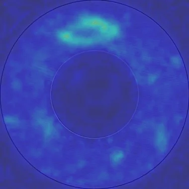
Seen through LIVE, the response on the same part bleeds across the whole ring; seen through 3D Surface it converges on the actual position of the defect (above is the 3D Surface side).
| ROC AUC | 0.935 → 0.970 |
|---|---|
| Overlap between good and defective scores | 0.37 → 0.06 |
| False alarm rate (at the optimal threshold) | 34.3% → 17.1% |
Values on a test set under identical conditions (n=128, a single part). They do not guarantee equivalent performance for every object or environment.
Where they sit
The methods, and the products.
The explanations are about method. The products are those methods made to work on a floor. Here is which of the three layers each belongs to.
FORESIGHT STEREO®
A 3D imaging technique developed from photometric stereo. From illumination in many directions it takes the surface normal, independently of the lighting, and recovers 3D shape. How the method works →
E3 ENGINE®
The anomaly detection engine. It learns from good products only and returns OK / Human_Check / NG. How the method works → Product page →
TR series
The systems that carry the sensor and the decision, chosen to suit the conditions on the floor. See products →
Contact
The quickest answer
is to image it.
Whether a method suits your object is settled by capturing it. Tell us the surface finish, the size of what you need to catch and the conditions on your line, and we will work it out with you.