
3D reconstruction
From the direction a surface faces,
assemble its height.
What Photometric Stereo produces is the direction the surface faces at each pixel. Joining those directions up into height is the step called 3D reconstruction. We integrate the gradient field as a whole, in one go.
Why isn't it enough to “add up from one edge”? And where does the error that integration introduces build up? This page is here so you can try both for yourself rather than read about them.
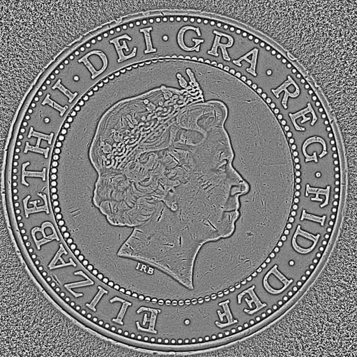

◀ Drag to compare ▶
One and the same capture. On the left, the surface direction; on the right, the product's 3D Surface output, made by integrating it into relief. On this page we follow nothing but this coin's normals, all the way through.
Experiment 01
Add from one edge, and streaks appear.
Solve it as a whole, and you get a shape.
The solid below is neither a photograph nor a CG model. We took the surface normals n measured by FORESIGHT STEREO, turned them into gradients (p, q), integrated them into height in your browser, and drew that height directly as a surface. Switch the integration method and drag to rotate it.
Integrated height (height in pixels; drag to rotate the viewpoint)
Integration method
×2.0
35°
55°
How far the gradient field is from “closing” —
The input is the coin's surface normal map (reduced to 512 px). The calculation runs on gradients reduced to 256 × 256, p = −nx/nz and q = −ny/nz; the whole-field solve follows the same approach as our own implementation. The solid places the height on a 128 × 128 grid and is shaded from gradients calculated from that height.
Why path integration leaves streaks.
Strictly speaking, a measured gradient field does not “close”. Going one pixel to the right and then down adds up to a slightly different height than going down and then to the right (noise, specular reflection and shadow are the causes). Add one row at a time, and these small mismatches build up separately in each row, turning into horizontal streaks. The answer changes with the path you choose ── that is the limit of path integration.
What solving the whole field at once means.
Instead of choosing a path, we search, for all pixels at once, for “the surface whose gradient closes and comes closest to the measured one”. Because it is solved in one go as a least-squares problem, the very choice of where to start adding disappears. The mismatch is not forced onto any particular path; it is spread thinly across the whole image.
* We implement this method on the GPU (as pre-processing for inference, the step that produces the 3D Surface output).
The equation
Pile up the slopes,
and you get height.
If the surface direction n = (nx, ny, nz) is known, the slope at that pixel (the rate at which height changes) is given by:
What we want is the height z whose slopes come closest to these (p, q). Rather than settling it pixel by pixel in sequence, we solve it for the whole surface together.
This way of solving has one property that cannot be avoided: the error collects at long wavelengths. Small errors in the gradient show up not as fine bumps but as gentle undulation across the whole surface. Experiment 02 below is there to measure exactly that.
Our implementation adds treatment before and after this solve (handling of the edges, removal of the overall tilt, normalisation for display, and so on). We do not publish the specific steps or constants.
A measured gradient does not “close”. Going right and then down, or down and then right, gives different heights for what should be the same pixel. Rather than choosing a path, we search for the surface that comes closest overall.
Experiment 02
Error builds up not in the detail,
but in the undulation.
Deliberately add a uniform tilt and noise to the normals, then integrate. The fine relief barely changes, yet the long-wavelength undulation moves a great deal. Then remove it, step by step, with the same “subtract a plane” and “remove undulation” that our implementation uses.
Top: shading of the integrated height Bottom: profile along the centre row (thin line = unperturbed result, thick line = perturbed result)
0.0°
0.0°
24 px
Deviation from the unperturbed result (RMS, pixels) —
of which undulation (long wavelengths) —
of which detail (short wavelengths) —
The tilt and noise are simulated (after converting the measured normals to p, q, the uniform tilt adds a constant, and the noise adds a normally distributed random value at each pixel). The “deviation” is the difference from the unperturbed result with the same post-processing applied, and the dividing line between undulation and detail is the wavelength on the slider (our implementation's default is σ = 30 px at the original resolution; here the calculation is reduced to 256 px, so the scale means something different). Height is in pixels, not physical units.
A 1° tilt becomes a slope across the whole surface.
Tilt the normals uniformly by 1°, and tan 1° ≈ 0.017 is added to the gradient. Over one pixel you see nothing, but piled up over 256 pixels it is a slope of about 4 pixels. The denominator in the equation above amplifies it ── error accumulates with distance and collects at low frequencies. That is why our implementation always subtracts a plane after integrating.
Choosing to keep only the detail.
Turn on “Remove undulation”, and all that is left is short-wavelength relief such as scratches and lettering. This is why our 3D Surface output brings out only the scratches, even on a warped plate. The flip side is that the warp of a whole plate, or absolute height, is not what this method is good at (→ Limits).
Four outputs
Before and after integration
are the product's outputs.
What you handled in Experiments 01 and 02 comes out of FORESIGHT STEREO as outputs, all at the same time, from a single capture.
The input to integration.
The n in the equation. (p, q) is made from it.
Integrated, with the undulation removed.
Corresponds to Experiment 02 with “Remove undulation” turned on. Only the fine relief remains.
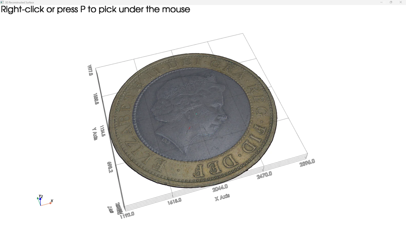
Turn the height as a surface and look.
The same thing as Experiment 01. Change the height exaggeration and viewpoint, and check the relief by eye.

The material's brightness, laid over the surface.
Held separately from shape, so it can be overlaid afterwards, like “Lay over the surface” in Experiment 01.
* Image 02 is the output of our product itself, not a result calculated on this page. The approach is the one described above in “Pile up the slopes, and you get height.” (the specific steps and constants are not published). The correspondence shown here explains the procedure; it does not indicate that pixel values match.
On the bench
Just change the lighting,
and it becomes 3D.
Experiments 01 and 02 were integrations solved in the browser. Do the same on the real system and, without moving the camera or the object, surface direction turns into height, becoming a solid you can rotate within a set of coordinate axes.
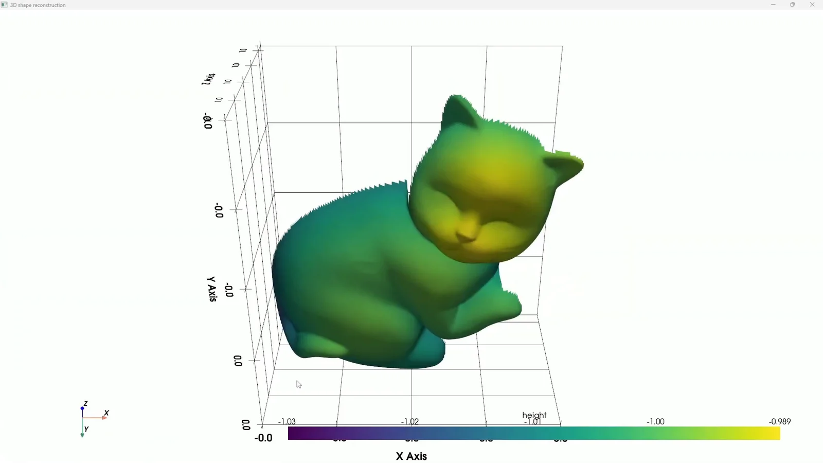 1:29
TOMOMI RESEARCH / YouTube Watch on YouTube ↗
The footage is real output from our own system. The video is in Japanese. Nothing is loaded from YouTube until you press play (at that point the player switches to youtube-nocookie.com).
Strengths and limits
The height you get from integration —
height of what, exactly?
The difference between adding from one edge and solving the whole field at once is what you saw in Experiment 01. But since both are ways of “assembling height from slope”, they also share some limits.
| Path integration | Solve the whole field at once | |
|---|---|---|
| How it solves | Fixes one path and adds the slopes in order | Solves all pixels together by least squares |
| Response to a gradient that does not close | Builds up separately along each path, becoming streaks | Spread thinly across the whole image |
| Computation | Proportional to pixel count, but hard to parallelise | Can be solved in one batch on the GPU |
| Boundaries | Depends on the choice of starting point | The edges need treatment |
| Shared limits | Only relative height is obtained / error collects at low frequencies (undulation, warp) / errors in the normals become errors in height as they are | |
* This is a general comparison of methods, not a statement of the performance of any particular product.
There are clear things it is not good at, too.
This method rests on two things: that the slope has been measured correctly, and that joining slopes together yields a surface.
What integration determines is the difference in height. The constant (where zero lies) is not determined, and the unit is a relative value that comes from per-pixel slope. Converting to μm needs the physical size of a pixel and a separate reference.
As Experiment 02 shows, error collects at long wavelengths. Warp across a whole plate, or large-scale shape, is a job for a different method such as triangulation. Our 3D Surface deliberately removes this component to keep the detail.
When specular reflection or shadow makes a normal lie, integration faithfully piles that lie up. Integration does not create error, but it does not remove it either. The remedy belongs on the side that solves for the normals.
Because the whole surface is solved together, how the image edges are handled changes the result. Our implementation adds treatment so that false steps do not rise at the edges, and smooths the borders of the mask before passing it on.
That is why we use 3D reconstruction not as “a tool for measuring dimensions”, but as a tool that turns relief buried in reflection into a form people and AI can see. Not guaranteeing the depth of a scratch in μm, but making the fact that a scratch is there stand up as shape ── that is the role of this step.
Where it sits
Where this step sits.
3D reconstruction is a step on the sensor side. It comes right after the step that solves for the normals (Photometric Stereo), and produces the 3D Surface output and the 3D view in Viewer.
FORESIGHT STEREO®
Captures the surface normal, illumination-invariant, from multi-directional lighting, and integrates it into height using the method on this page. Solving for the normals →
E3 ENGINE®
An AI anomaly detection engine that learns only from good parts and puts a number on how far a part departs from them. 3D Surface can be selected as its input. How the judgement works →
TR series
The sensor and the judgement, combined into a single unit that runs on the shop floor. The benchtop observation unit TR-55 comes with Viewer, for rotating and examining this 3D view.
* The standalone software AI SMART MASK sits outside these three layers (it is pre-processing that decides “where to look”, and it does not make OK / NG judgements).
Related
Products where this step is at work
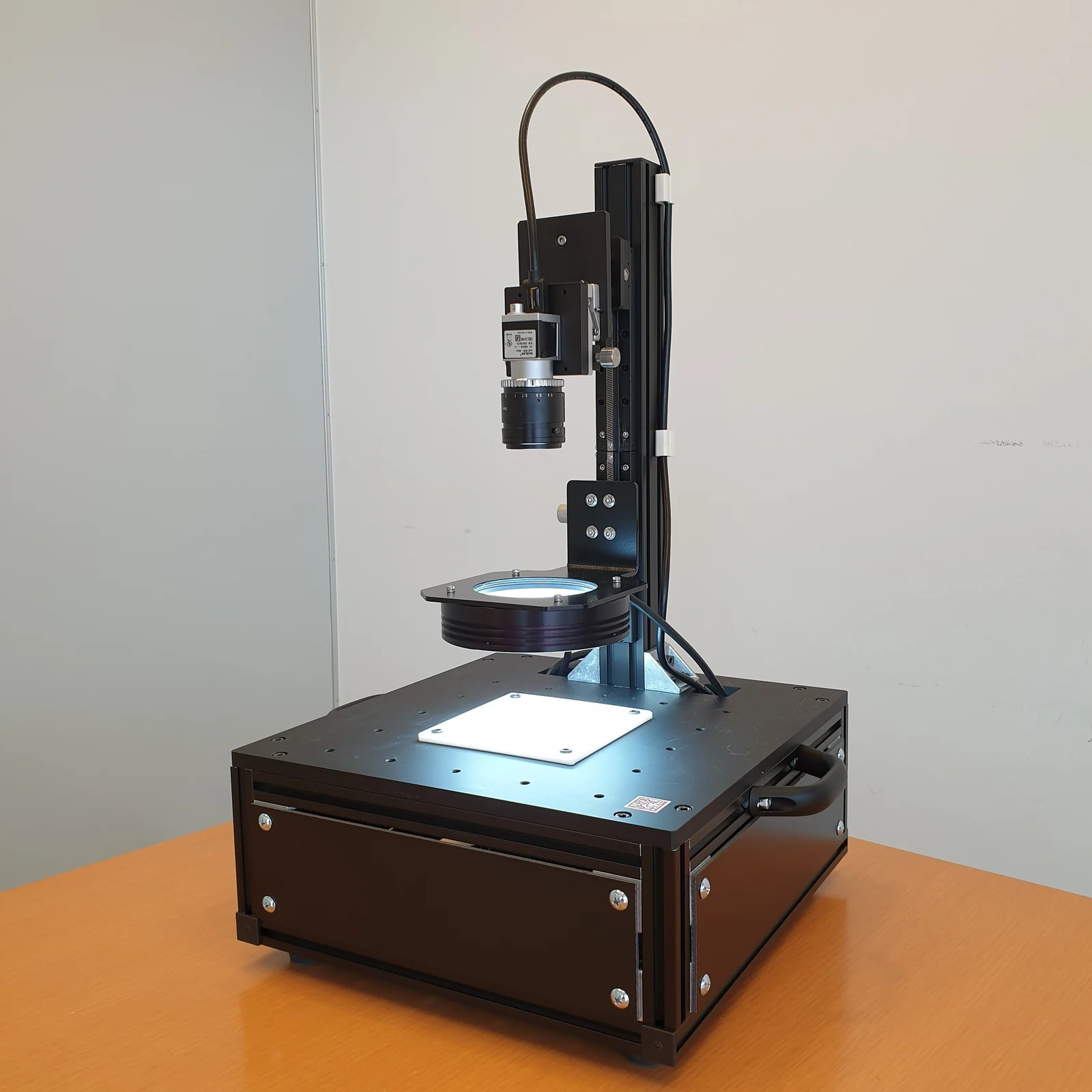
Place the sample and press a button for four outputs and a 3D view. Experiment 01's “turn it and look”, on your own sample at hand.
Read more →
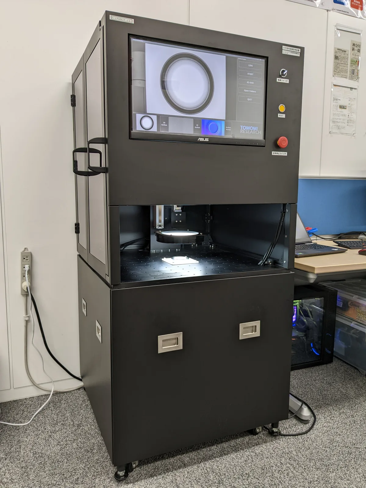
A configuration that fits everything from capture to judgement into one unit. 3D Surface can be selected as the input for judgement.
Read more →
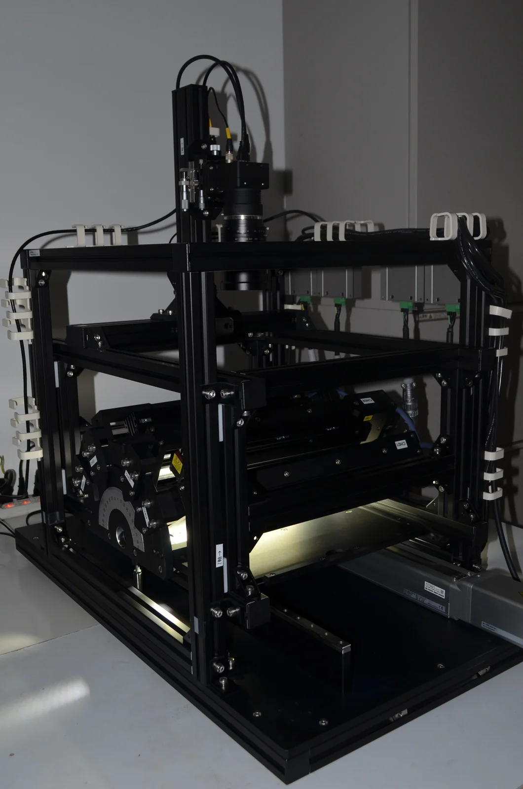
A continuous inspection system that captures on a moving line and produces the 3D Surface right there.
Read more →
Contact
On your object,
will the relief stand up?
Whether it does is decided by the surface finish, and by the height and wavelength of the defects you need to see. A screen can only take you this far. Start by sending us a sample: we image it and send back the 3D Surface and the 3D view in Viewer.