
Anomaly detection
Learn from good products only,
and notice the difference.
Instead of collecting examples of defects and teaching them, anomaly detection learns from good products only and turns the distance from them into a number. It is also the idea at the core of our anomaly detection engine, E3 ENGINE.
What does “no need to collect defects” actually mean? And where, even so, are defects needed? This page is here so that you can try both for yourself, rather than just read about them.
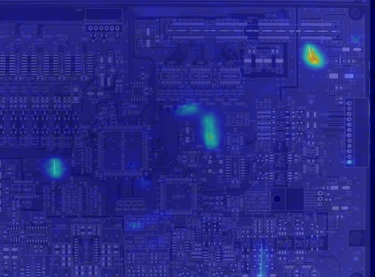
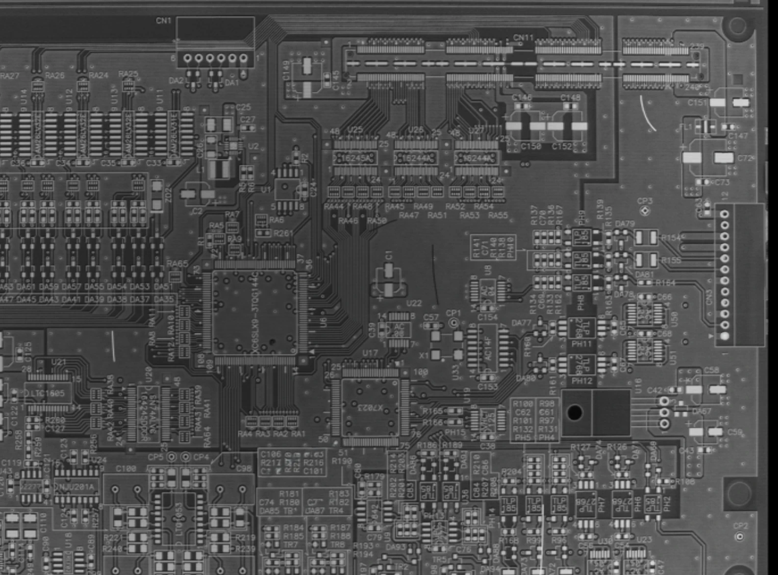
◀ Drag to compare ▶
A printed circuit board from a real project. Actual output of E3 ENGINE trained on 122 good images only: anomaly score 0.45 (threshold 0.169), verdict NG. The experiments that follow reproduce this mechanism in a simplified form so that you can handle it.
Experiment 01
The more good products it remembers,
the quieter good products become.
The blue surface below is not a photograph. Using concrete images from a public dataset, your browser computes, on the spot and for each small window of the input image, “the distance to the nearest of the good-product windows in memory”, and shades each place more deeply the larger that distance is. Right now it has memorised 16 good images. Reduce the number it remembers, and then switch to sound surface D.
Computed anomaly map (place the pointer on the image and the list on the right shows the “nearest good window” for that spot)
Test image
16 images
±0 %
What happens if you capture at a brightness different from the good products in memory?
Image score (mean of the top 1% of window scores) —
Furthest window —
Good images in memory (faded ones are not memorised yet)
The input is 20 images of 227 px (17 good, 3 with cracks) from the public dataset “Concrete Crack Images for Classification” (Özgenel, Ç.F., 2018 / Mendeley Data / CC BY 4.0). The computation works on greyscale images reduced to 96 px: windows of 5 × 5 pixels are cut out every 2 pixels, and the distance to every window of the good images in memory is found exhaustively (no approximation). The depth of the blue is on a fixed scale that saturates at a distance of 0.6.
What is happening.
When it remembers only 1 image, even sound surface D is painted blue. Patterns and brightness not in its memory are treated as the same “unknown” as a crack. As you increase the number it remembers, the sound surface goes quiet and only the cracks remain. Remembering the variation among good products is what learning means in this method.
Now shift the brightness. The further you move towards the dark side, the bluer even the sound surface becomes. A brightness not in memory cannot be told apart from an anomaly — which is why, when the imaging conditions change, you do not reuse the same model; you train it again.
How E3 ENGINE differs.
Here, the feature is the pixel values of the window themselves. E3 ENGINE measures the same distance using features extracted by a trained neural network, so it is far less sensitive to fluctuations in pattern and differences in brightness, and sensitive to “differences in structure” such as cracks.
What they share: only good products are memorised; the nearest match in memory is searched exhaustively; and the score of one image is set as the mean of the top 1% of window scores. The skeleton of the mechanism is the same.
* Neither the object nor the images are things we inspect; they are public data used to show the mechanism. For real examples on our systems, see the circuit board above and the enamelled wire below.
For those who would like to move “where OK and NG are split” themselves once the scores are out — a demo in which you can move the distributions and the threshold in your browser is published as LAB on our Japanese site.
The principle
Measure the distance from “normal”,
window by window.
Images of good products are divided into small windows, and the features of each are kept as a memory. The input image is divided into the same windows, and for each window the distance to “the nearest good-product window in memory” is measured. That distance is the anomaly score at that place.
M is the memory of good products, and f is the function that extracts features from a window. Laying the distances out over the image gives the anomaly map. The mean of the top 1% of the map becomes the image score, which is compared with a threshold to reach a verdict.
No defect images appear in training. Because it has not been taught what a defect “looks like”, distance rises even for kinds of defect nobody anticipated. In return, brightness and patterns that good products do not have raise distance in just the same way — and this decides both its strengths and its weaknesses.
When E3 ENGINE builds its memory, it compresses it by keeping only representative points that lie far from one another (by default, 10% of the whole), and at inference it searches for the nearest neighbour exhaustively, without an approximate index. It puts answers that do not change ahead of speed.
Place the input window in feature space and measure the distance to the nearest point in the memory of good products. Windows that resemble good products are a short distance away; what good products do not have is a long distance away.
Experiment 02
To draw the line,
you need real defects.
Training needs good products only. But “from where on do we call it NG?” cannot be decided from the scores of good products alone. On the scores of 18 images measured in the same real project as the circuit board above, move the two boundaries yourself.
Measured scores for 18 images from a real project (13 good, 5 defective). Move the boundary lines by dragging them on the chart or with the sliders below.
Data
—
—
Good, 13 images —
Defective, 5 images —
The real-project scores are evaluation output from E3 ENGINE Trainer (printed circuit board, trained on 122 good images, image size 1024, 2026-02-12). The 5 defective scores are the values in results_summary.csv; the 13 good scores were read from the evaluation plots to two decimal places. The dashed line is the optimal threshold calculated by Trainer, 0.169. The public-dataset distribution was read from Trainer's histograms (bins of width 0.005 / 0.007), and all proportions are approximate. The 4,000 good and 20,000 defective images are each normalised by their own total.
Human_Check is not a way out.
Between the highest good score and the lowest defective score lies a band that cannot be called either way. E3 ENGINE separates it out as Human_Check and returns it to the human eye. A wider band means fewer misses and fewer false alarms, but more images for a person to look at. Where to draw the line is a decision for the floor, not for the machine.
Switch to the public dataset and you get a feel for what happens when the hills of good and defective overlap. Move one boundary, and the other figure always moves.
That is why evaluation needs defects.
Tick “Hide the real defects”. The upper limit of the good scores is visible. But where above it to draw the line so that the defects fall beyond it simply cannot be decided without having seen a single defect.
Good products are enough for training. But calibrating the threshold needs evaluation data that includes both good and defective pieces. Not confusing these two is the first rule for using this method on the floor.
What to feed
The same mechanism gives a different answer
depending on what you show it.
What anomaly detection picks up is “whatever differs from memory”. So what you feed it as input decides the result. These are score maps for the same enamelled wire: trained and judged on Live, as the human eye sees it, and trained and judged on the Surface Normal of FORESIGHT STEREO®.
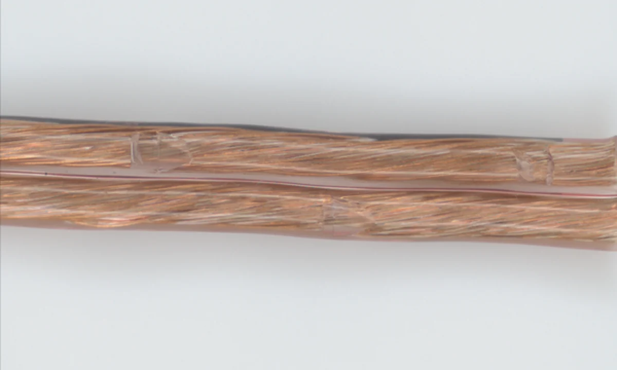
The image just as the human eye sees it.
The fluctuating gloss goes into the “memory” as it is.
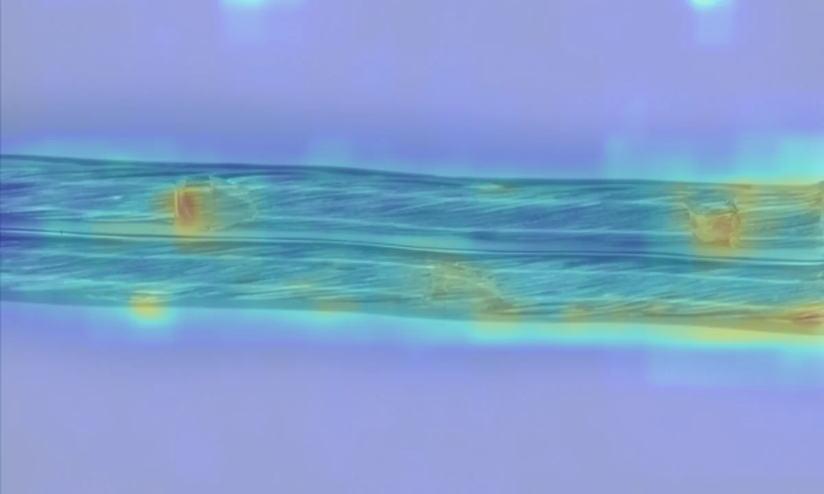
The response spreads beyond the damage.
It does respond to the damage. But warm colours also sit on the sound strands, and it cannot narrow down where to look.

The orientation of the surface, encoded as colour.
A physical quantity that does not depend on the lighting. Fluctuating gloss does not enter; only disturbances in shape remain.
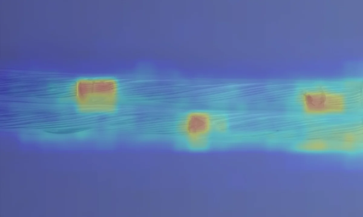
The response stands on the damage alone.
When only shape goes into memory, distance rises only for anomalies in shape.
* Measurement conditions — Surface Normal: trained on 63 good images; evaluated on 14 good and 7 defective. Live: trained on 61 good images; evaluated on 10 good and 7 defective. Because the numbers of training and evaluation images differ, this is not a strict comparison in which only the input was swapped. It is what was observed on this one sample, and does not show that the same difference appears on every object. Which output to feed is confirmed on samples for each object. How Surface Normal is measured: see the photometric stereo explainer →
On the bench
Having learnt good products only,
what comes back?
What E3 ENGINE actually returns is three things: a label, a score and an anomaly map. The threshold you placed in Experiment 02 is what decides where the line falls on that score.
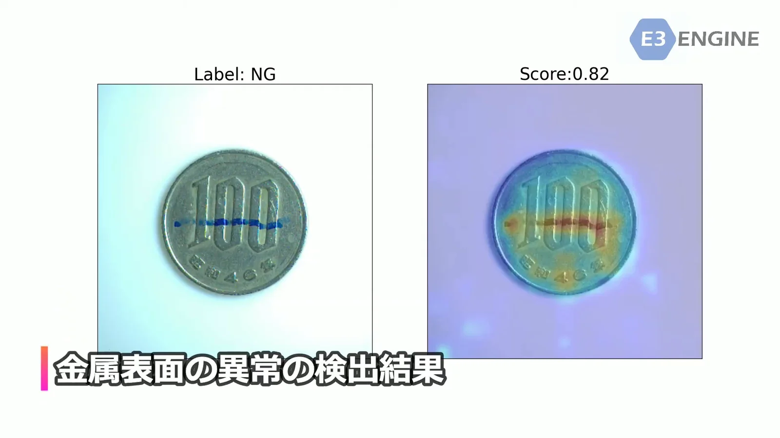 0:31
TOMOMI RESEARCH / YouTube Watch on YouTube ↗
The footage is the screen of our own system, filmed by us. The video is in Japanese. Nothing is loaded from YouTube until you press play (at that point the player switches to youtube-nocookie.com).
Strengths and limits
The other side of
not teaching defects.
Anomaly detection that learns from good products only and classification taught from collected defects are exact mirror images in what they do well and what they do poorly.
| Anomaly detection, learning good products only | Classification, taught from collected defects | |
|---|---|---|
| What training needs | Images of good products only | Good products, and defects labelled by type |
| What it returns | An anomaly score, and a map of where it differs | A classification: which type of defect it is |
| Unanticipated defects | Distance rises for anything good products do not have | Types it was not taught cannot be judged |
| Variation in good products | Variation not in memory also shows up as an anomaly (retraining when imaging conditions change) | Can be absorbed if within the range included in training |
| Threshold | Calibrated on evaluation data that includes good and defective pieces | The classifier's output can often be used as it is |
* This is a general comparison between methods and does not show the performance of any individual product. What can be found depends on the object, the imaging conditions and the variation among good products.
There are clear weaknesses, too.
This method stands on the premise that “anything good products do not have is an anomaly”. As you saw in Experiments 01 and 02, that premise gives up a few things in exchange for its convenience.
What comes back is “how far from good products” and “where”. It does not judge whether it is a scratch, a stain or a chip. If you want to sort by type, a separate job is needed downstream of this mechanism.
When the lighting, the angle or the line changes, good products also move away from memory. What happened when you shifted the brightness in Experiment 01 happens on the floor as a change in imaging conditions. When conditions change, the assumption is that a separate model is built again.
Good products are enough for training, but the boundaries dividing OK / Human_Check / NG are calibrated on evaluation data that includes good and defective pieces. As Experiment 02 showed, the line cannot be placed without seeing a single defect.
Distance is measured window by window, so differences finer than the window's granularity are diluted across the whole window. To pick up fine defects you raise the image size and make the windows finer, but memory and computation get heavier by the same measure (guide for E3 ENGINE: 512 px needs 4 GB VRAM or more, 768 px 6 GB or more, 1024 px 8 GB or more).
What we have worked hardest on before anomaly detection is making 02 and 04 even a little easier. Feed it Surface Normal, which does not depend on the lighting, and there is less “brightness not in memory”, while shapes that were buried in reflections stand out as distance. Change what is looked at before changing the algorithm — that is our order of things.
Where it sits
Where this method sits.
Anomaly detection is a method, not a product name. Among our products, the one that carries this method is Layer 02 of the three layers.
FORESIGHT STEREO®
A 3D imaging technique developed in our own way from photometric stereo. From illumination in many directions it takes the surface normal, independently of the lighting. The layer that makes “what is looked at” for anomaly detection. See how it works →
E3 ENGINE®
The AI anomaly detection engine that implements the method on this page. It learns from good products only and returns one of three verdicts: OK / Human_Check / NG. Product page →
TR series
The sensor and the decision, brought together in a single unit that works on the floor. From benchtop observation units to continuous inspection systems on the line and robot-mounted systems.
* The standalone software AI SMART MASK sits outside these three layers (it is pre-processing that decides “where to look”, and does not judge good or defective).
Related
Products that run on this method
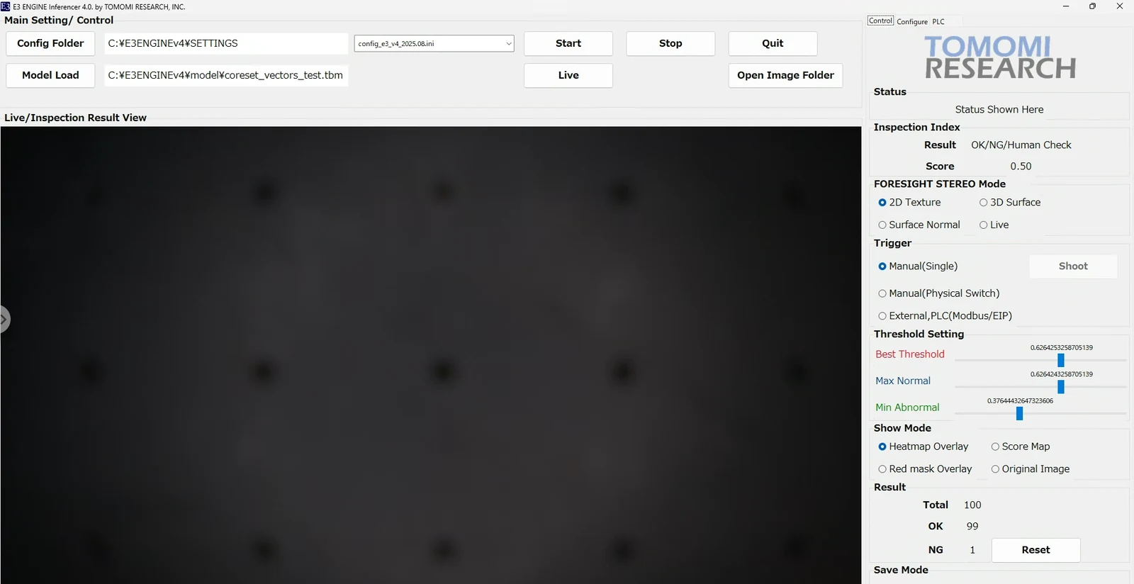
The method on this page itself. Three applications for training, evaluation and inference, with measurements from real projects.
Read more →
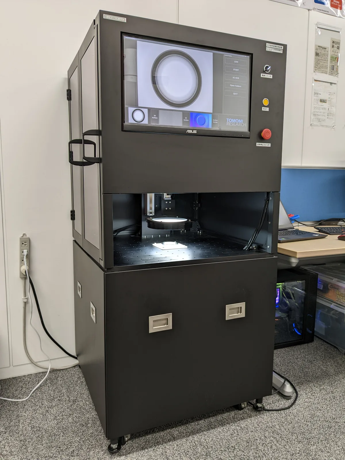
Imaging through to the verdict in a single unit. The enamelled wire above was measured on a system of this family.
Read more →
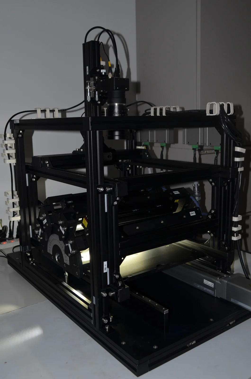
A continuous inspection system that captures on a moving line and returns the verdict on the spot.
Read more →
Contact
Do your good products
separate from the defects?
Whether they separate depends on the object, the variation among your good products and the state you want to find. This is as far as a screen can take you. Start by talking to us: we take your images of good products, train on them, and show you how the scores separate on your real defects.