
Resolution
Whether a small scratch shows
depends on the size of one pixel.
“How small a scratch can it see?” ── it is the question we hear most in sales meetings. The answer does not start with the name of a system. It starts with a single division: field of view ÷ pixel count.
On this page we take one measured image, make it coarser step by step, and see what that division means. The image is our own output of a British £2 coin. The coin’s 28.4 mm diameter serves as the ruler, so how many μm one pixel of this image covers is fixed by measurement, not by estimate.


◀ Drag to compare ▶
The right is the measurement itself (21.4 μm per pixel). The left is the equivalent of 171 μm per pixel, made by averaging that same image in blocks of 8 × 8 pixels — it is not a second photograph. Both show the same place, an area 16.5 mm square.
Experiment 01
Place one pixel on the real object.
Only two things decide it: how wide an area you capture (the field of view) and how many pixels the camera has across. Together they set the real size each pixel covers.
The image below is recalculated from the measured image to show how it would look if captured at the pixel size you have chosen. Enter the width of the defect you want to see, and it tells you how many pixels it spans.
The source image is 21.4 μm per pixel. Choosing a finer setting cannot draw it any finer than the source (what is not there cannot be shown).
300 mm
300 μm
Real size covered by one pixel 73.2 μm
Pixels the defect spans 4.1 pixels
The shape appears. Position and size can both be read.
How the ruler for this image is set.
Fitting a circle to the outline of the coin in the image gives a diameter of 1325.4 pixels (fit residual 0.67 pixels). The Royal Mint publishes the diameter of the £2 coin as 28.4 mm, so one pixel = 21.4 μm.
The whole image is 1640 × 1360 pixels, so the field of view is about 35 × 29 mm. This value changes with the lens and configuration, so the field of view and resolution of each model are still to be confirmed in the specifications.
“Coarsening” means averaging.
What happens here is that the source image is averaged by area over the extent of each new pixel. A real camera does the same: each pixel gathers the light that reaches its area into one value.
※ Lens blur (soft imaging) is not included. The real thing comes out softer still than this calculation. In other words, what you see here is the best you can hope for at that pixel count (→ When there are enough pixels and it still does not show).
The arithmetic
One division.
Then come the conditions.
For a first answer on resolution, these two lines are enough. The hard part comes after: how many pixels it takes before you can say “something is there”.
A defect smaller than one pixel only shifts the value of that pixel slightly, and does not stand out from its surroundings. With two pixels you can tell that “something is there”, but no shape appears. To see a row of structures as separate, two pixels per period is the theoretical limit (the sampling theorem), and at that point contrast falls to a quarter of the original. Experiment 02 measures this.
When practitioners say “secure three to four pixels”, they are leaving a margin against this fall-off.
Widen the field of view three times without changing the pixel count, and the real size of one pixel triples too. The same defect goes from 3 pixels to 0.3 pixels and no longer remains as a difference from its surroundings.
Experiment 02
Where dots stop being dots.
On this coin, the edge surrounding the portrait carries a ring of evenly spaced dots, 0.54 mm apart (113 to a full circle; values measured from the image). Because the spacing is known, we can follow in numbers the point at which they become a single line.
Move the slider to make one pixel larger. On the left is the image; on the right, the contrast of the dot ring measured on the spot. The pictures are not being swapped: the contrast is measured afresh every time on the coarsened image. What is measured is the amount of tilt in the surface orientation (the normal). The dots are “shape”, so they show more strongly in the normal than in brightness.
The blue arc marks where the contrast is measured (it follows the ring of dots around the portrait).
The vertical axis is a proportion of the original (21.4 μm per pixel) taken as 100%. The dot marks the current setting.
21.4 μm
Dot spacing 26.0 pixels
Contrast 0.50
Against the original 100 %
The dots stand apart as dots.
Nyquist is a limit, not a target.
To see two neighbours as separate, two pixels per period (= one pixel per dot) is the theoretical limit. But take it that far and the measured contrast is a quarter of the original — thin enough to be buried in noise or uneven lighting.
Keep four pixels per dot (a period of 8 pixels) and about 70% remains; at two pixels (a period of 4 pixels), about half. With the representative TR-300 configuration (8K, 100 mm field = 12.2 μm per pixel), this “4 pixels = 70% remains” level corresponds to a width of about 49 μm. Widen the field to 300 mm with the same camera and one pixel becomes 36.6 μm, putting the same level at about 146 μm. This is why the smallest defect size does not come down to one number.
Do not rely on values around 2–3 pixels.
Around this part of the graph, the value bobs up and down instead of falling cleanly. Whether the row of dots and the pixel grid happen to line up or not changes what you see (aliasing).
It is the zone where, even with the same object, a slight shift in placement flips “seen” and “not seen”. Set the inspection conditions here and the results will vary from day to day.
In numbers
Resolution is not one thing.
When someone asks “what is the resolution?”, there is more than one number to give. Depending on how the image is captured, several resolutions, each set in a different way, exist at once.
Field-of-view width ÷ pixels across — the division this page has been about. It is set by the lens and the pixel count, and does not move unless the system configuration changes.
The distance the workpiece travels while one line is captured. It is set by conveyor speed ÷ line rate, so it is a different value from the across direction. If the conveyor speeds up, only the along direction gets coarser. Line scan explained →
This is set independently of the in-plane resolution. Our 3D Surface is a relative height, and cannot be read as an absolute value in μm. 3D reconstruction explained →
Before the verdict, captured images are resized to a square of a fixed pixel count for training and inference. Even if the capture is fine enough, it coarsens once more at this stage. What coarsens, and by how much, is shown in the table below. What happens when it is handed to the verdict →
Why we do not give the smallest size as one number.
| Cameras | 2K / 4K / 8K / 16K line scan supported Source: TR-300 specifications |
|---|---|
| Imaging width | Set to suit the application Source: TR-300 specifications |
| Resolution across | About 12.2 μm/pixel (with 8K and a 100 mm field. Theoretical value: 8,192 pixels assigned to a 100 mm width) |
| → Width spanning 4 pixels | About 49 μm (12.2 μm × 4. Our conversion. The “70% remains” level of Experiment 02) |
| → With the field widened to 300 mm | About 36.6 μm per pixel / the same level at about 146 μm (still 8K. Our conversion) |
| Minimum detectable anomaly | Depends on imaging conditions and defect shape Source: TR-300 specifications. Not published as a single number |
| Lighting directions | TR-300 = 4 directions / TR-100 = 8 directions |
| Processing time | 30 ms (up to generating the 3D image; 4MP × 4 images; RTX 3060 6GB) 60–80 ms (representative processing time including the AI verdict) |
| Field of view and resolution by model | 〔要確認〕 Not published for TR-55 / TR-100 / TR-500 |
We do not publish the minimum detectable anomaly size as a single number because it is set by the resolution and the shape of the defect. As the table shows, even on the same system the answer changes threefold once the field of view is decided. What needs deciding before any catalogue figure is how wide an area to capture, and with how many pixels. These are TR-300 values and cannot be generalised to other models. 12.2 μm/pixel is a theoretical value and does not include lens blur (MTF).
Handed to the verdict, it coarsens again.
So far this has been about the capture side. Captured images are not passed to the verdict as they are. Our anomaly detection engine (E3 ENGINE) resizes them to a square of a fixed pixel count before working on them. Even if the capture resolution is sufficient, it drops once more at this stage.
| 1. Resize to a square | The image is scaled up or down to a square of a fixed pixel count. The aspect ratio is not preserved,
so a wide capture shrinks more strongly across. Defaults: 512 pixels (Trainer standard) / 256 pixels (Simulator default). Set per project |
|---|---|
| 2. Trim the four edges | The edges are cut off by the crop amount before the image is passed on. At 512, 8 pixels → 496 × 496 / at 256, 16 pixels → 224 × 224 |
| 3. It becomes a map of scores | The anomaly map is not as fine as the input pixels. At the stage where features are extracted,
it becomes a grid 1/8 the size of the input. 496 × 496 → 62 × 62 / 224 × 224 → 28 × 28 (measured on our implementation) |
Pass the capture used on this page (1640 × 1360 pixels, 21.4 μm per pixel) to the 512-pixel setting, and it becomes 3.2 times coarser across and 2.7 times coarser vertically: one pixel is equivalent to 69 μm / 57 μm. In terms of the original capture, each cell of the 62 × 62 score map corresponds to 0.57 × 0.47 mm.
※ This does not mean that a defect smaller than one cell “cannot be detected”.
A change inside a cell affects its features, so the score can still rise. What coarsens is
the precision of “where it is”.
※ Put the other way round, if the area you want to see is only part of the field of view, cutting out just that area before the verdict
lets the same 512 pixels be spent on it. That is what pre-processing that decides “where to look” is for
(→ AI SMART MASK).
Source: our anomaly detection engine’s implementation (working source code). The grid sizes were confirmed by actually running it.
On the bench
When a line finer than a hair
lands on one pixel.
Footage of our system aimed at a 500-yen coin. The microtext “500YEN” hidden in the denomination, and the fine lines fanning out around the characters for “Japan” ── machining invisible to the naked eye rises up as surface orientation. Whether it shows this far is decided by the division on this page.
 1:09
TOMOMI RESEARCH / YouTube Watch on YouTube ↗
The footage is real output from our own system. The video is in Japanese. Nothing is loaded from YouTube until you press play (at that point the player switches to youtube-nocookie.com).
Limits
Enough pixels,
and it still may not show.
Experiments 01 and 02 showed the ideal case of “coarsening the pixels and nothing else”. In reality, other factors cut in before that. A pixel-count estimate is a ceiling, not a promise.
Making the pixels smaller does not bring detail back if the image itself is soft. Before adding pixels, you need to check that the lens can actually resolve that fineness.
The range in focus is finite. If the workpiece has differences in height, the near and far parts look different. The higher the magnification, the narrower this range becomes.
Resolution is about whether things can be separated; whether they can be noticed is another matter. If the difference from the surroundings is smaller than the noise, it is buried however many pixels it spans. We measure surface orientation precisely to create a difference where brightness shows none.
Even if it is in the image, the verdict will not necessarily pick it up. The input resolution of the verdict, the variation of the good parts it learned and where the threshold is placed are separate factors.
Four ways to make one pixel smaller, and what each costs.
| Narrow the field of view | The surest way. But less area is covered per capture, so the same workpiece takes more captures |
|---|---|
| Use a camera with more pixels | Finer while keeping the field of view. In exchange, the data per image and the processing time grow |
| Change the lens | This is what works when the imaging is not keeping up with the pixels. The depth that stays in focus becomes narrower |
| Capture in sections | Split the field of view, capture several times and stitch afterwards. This needs positioning accuracy and takt time |
Which to choose depends on the size of the defect you want to see, the dimensions of the workpiece and the takt of the line. Talk to us, starting with us taking your object, actually capturing it and putting the required pixel count into numbers.
Where it sits
Resolution is set
by the very first layer.
Of the three layers, in-plane resolution is set by the sensor layer. The later layers only inherit the fineness set there; they cannot add to it.
Field of view, pixel count, lens and lighting. The real size of one pixel set here is the ceiling for everything that follows.
Returns a pass/fail verdict on the images it receives. Because it resizes them to a fixed pixel count first, they may coarsen once more here.
The form in which field of view and takt are set to suit the floor. Even with the same method, the real size of one pixel changes from model to model.
Related
Where the numbers come from
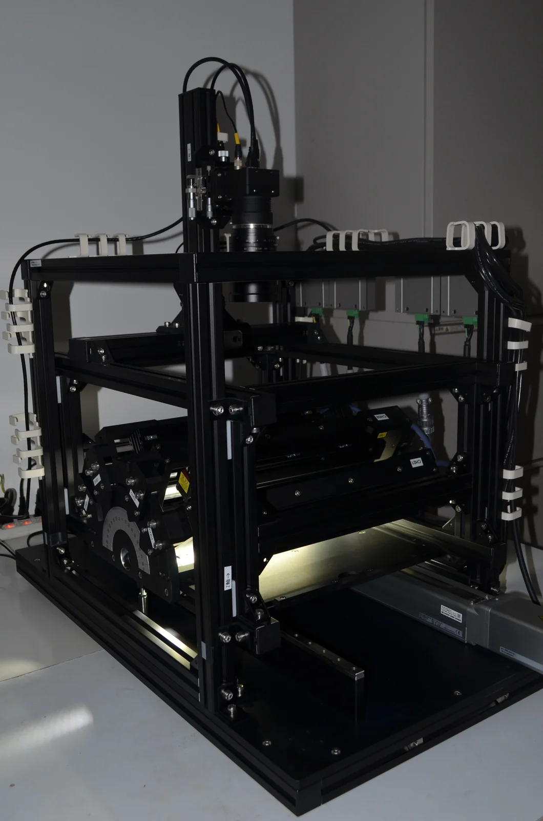
The source of the representative configuration used on this page (8K, 100 mm field = 12.2 μm/pixel).
Read more →
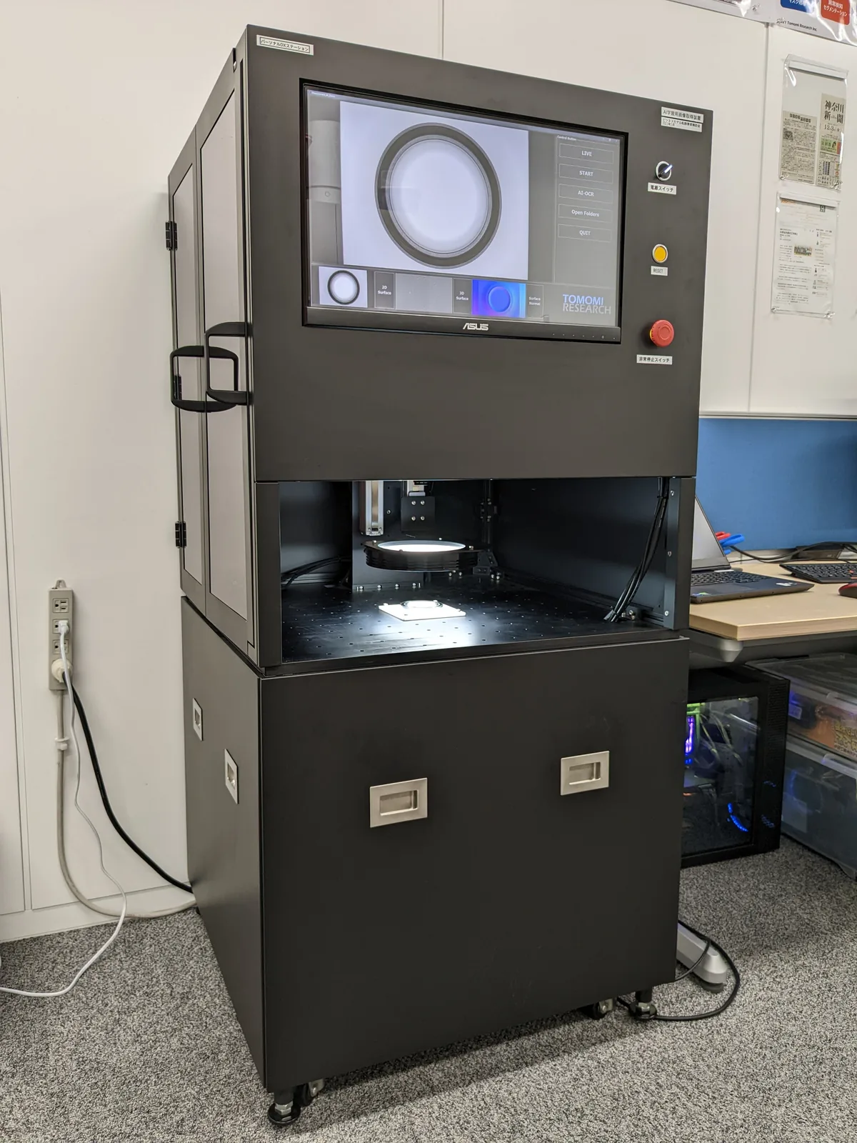
Capture through verdict in a single unit. The field of view follows the sample placed in it.
Read more →
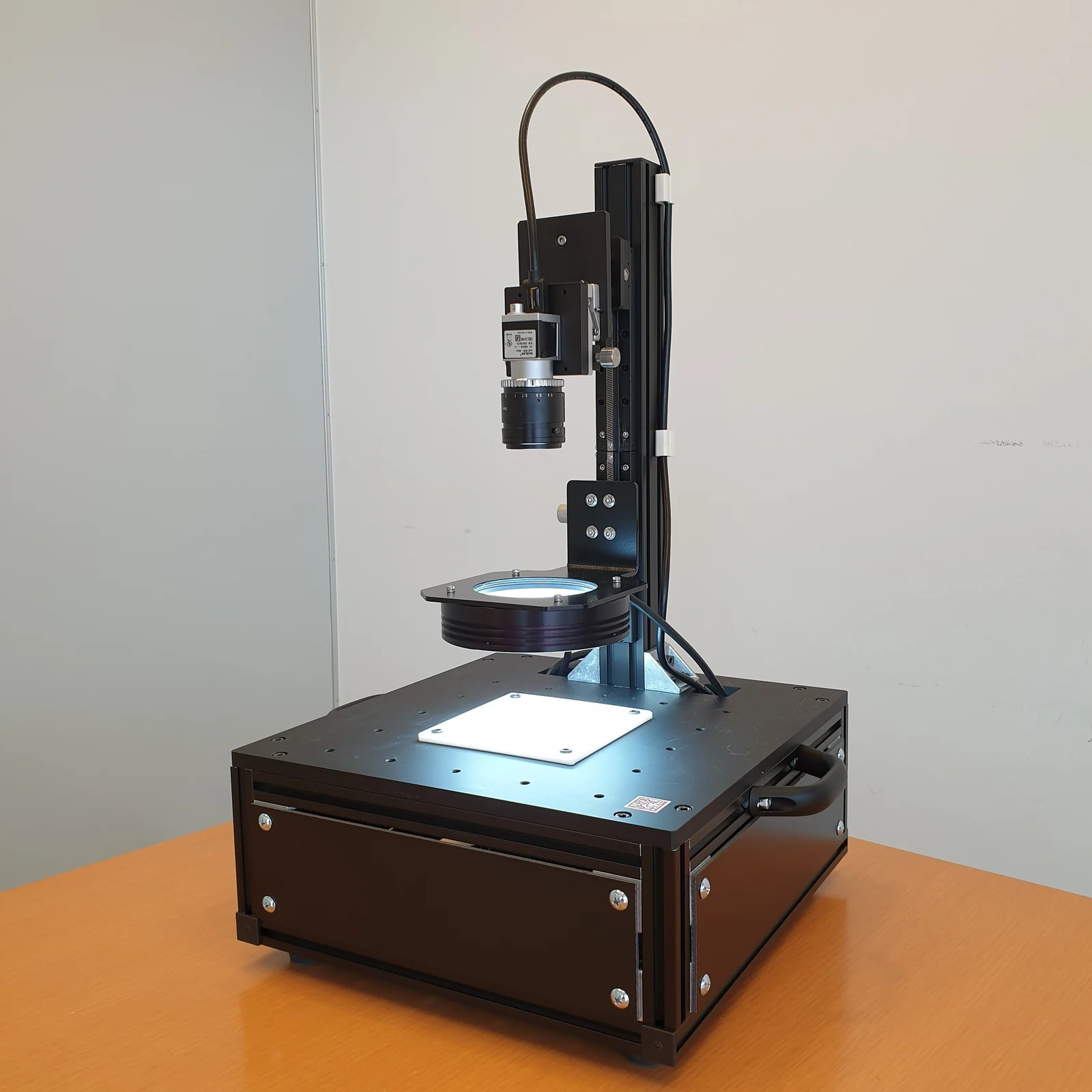
A unit for checking your own samples first. Actually capturing and counting the pixels is the quickest way.
Read more →
Contact
How many pixels
does your defect need?
The size of the defect you want to see, the dimensions of the workpiece and the takt of the line. Once these three are fixed, the required pixel count can be calculated. Talk to us, starting with sending us samples: we capture them and tell you how many pixels they show up at.