
Evaluation
“What is the accuracy?”
Why we don't answer with one number.
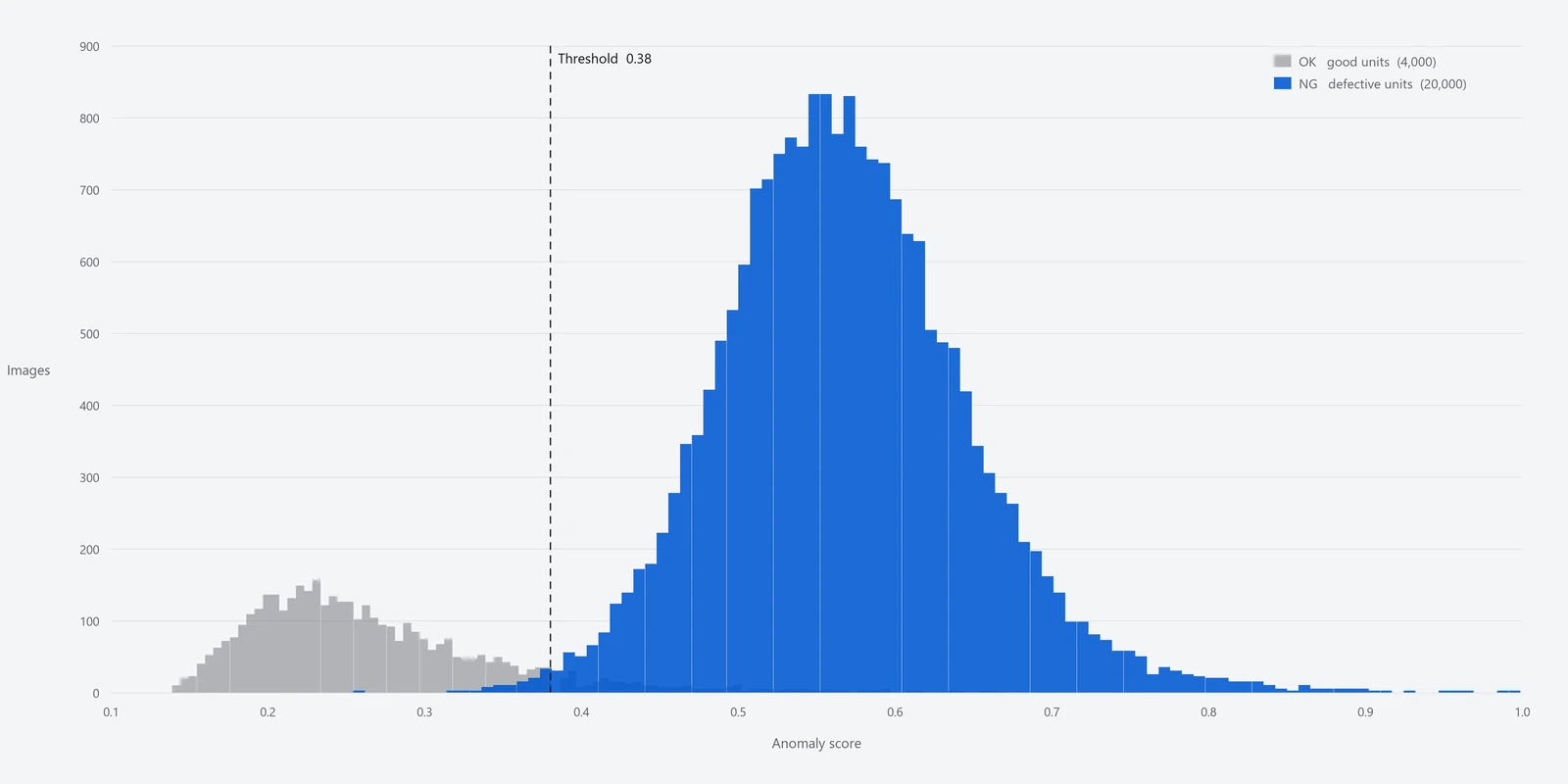
Same images, same model: the answer changes with where the line is drawn. So we answer not with one number but with the distribution, the operating point and the population.
This page is here so that you can check, against a real evaluation output and calculations done on the spot, how to read the numbers from an evaluation and what happens once the system goes into service.
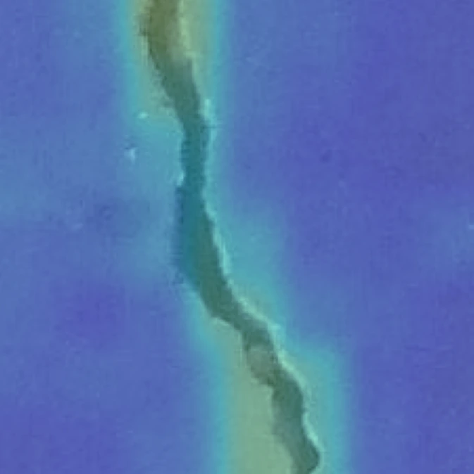
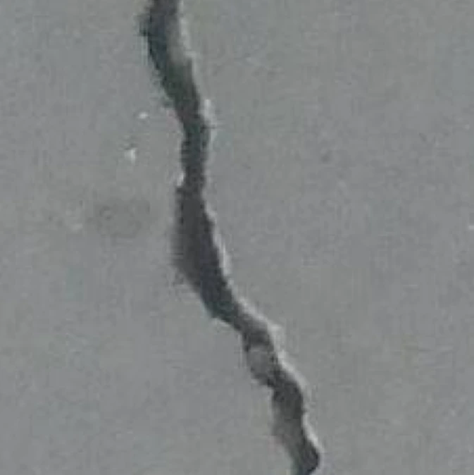
◀ Drag to compare ▶
The anomaly score of this image is 0.55. With the threshold at 0.38 it is NG; at 0.60 it is OK. Neither the image nor the model has changed.
Experiment 01
Misses and false alarms
do not fall together.
Lower the threshold and misses fall, but more good pieces are called NG. Raise it and the reverse happens. No setting brings both to zero at once.
Below, you move the threshold over the score distribution from our evaluation on a public dataset, and it is multiplied by the defect rate on your line and the daily output to turn it into actual piece counts.
The closer to the lower left, the better the setting. You can only move along the curve.
| Judged OK | Judged NG | |
|---|---|---|
| Actually good | — | — False alarms |
| Actually defective | — Misses |
— |
—
0.38
1.0 %
Miss rate (of defective pieces) —
False-alarm rate (of good pieces) —
Precision (real defects among NG) —
The curve is an approximation, drawn from a distribution read off the histogram of our evaluation output on the public dataset Özgenel (2018) Concrete Crack Images for Classification (Mendeley Data V2, CC BY 4.0). The ◯ in the chart is the measured point: the confusion matrix of the evaluation output itself (threshold 0.38; 291 of 4,000 good images judged NG = 7.3% false alarms; 97 of 20,000 defective images missed = 0.49%). The curve and the ◯ differ slightly, by the error of the reading. The defect rate and the daily output are assumptions you set.
Try lowering the defect rate.
Set the defect rate to 0.1% and the NG bin fills up with almost nothing but good pieces. Nothing about the model has changed. The only thing that changed is the population.
“It says NG, but what comes out is all good pieces” — when you hear this on the floor, this is usually why. Even with a low false-alarm rate, it happens when defects themselves are rare.
Which to favour is decided by the process.
Where an escape is critical, misses are kept to a minimum and false alarms are sent back by hand. Where a defect will be caught in a later step, the setting leans towards fewer false alarms and less handling.
This call is not made by the equipment. It comes from weighing the loss when a defect escapes against the effort of a person re-checking one piece. That is why we do not choose the operating point on our own.
※ What you can move here stops at assumptions such as the defect rate; the distribution itself is fixed to our measured values. If you want to build the distribution yourself and try ways of setting the threshold as well (maximum F1 / zero misses first / a cap on the false-alarm rate / minimum cost on the floor), there is a demo we publish for that — LAB.
Four numbers
Four numbers,
saying different things.
A single evaluation yields at least four “rates”. All of them are correct, and each says something different.
The denominators differ. The miss rate and the false-alarm rate depend only on the model and the operating point, but precision and accuracy move with the defect rate on your line.
On a process with a defect rate of 0.1%, judging everything OK is enough to reach an accuracy of 99.9%. High accuracy is no evidence that anything was found.
Rates taken from the same table say different things when their denominators differ. What gets called “accuracy” in a sales meeting is usually one of these.
Experiment 02
Five out of five
does not make “99%”.
When few defects are used in an evaluation, the spread of the resulting number is wide. Below, the range the true detection rate can fall in (the 95% confidence interval) is calculated from the number of defects detected.
This is settled by arithmetic alone and has nothing to do with how good the model is. It is why, when asked “if you have a track record, give us the accuracy”, we talk about sample counts first.
5
0
Apparent detection rate —
95% range of the true detection rate —
—
How many samples “99% or more” takes.
Assuming not a single defect was missed, pushing the lower bound of the true detection rate past 99% takes around 500 samples (with 500, the lower bound is 99.2%). With 100, you can only say 96.3%.
The real-project measurements published on our site are on the scale of 5, 7 or 9 defective samples. From those, “100% accuracy” cannot be written. We do not write it because it cannot be written.
When the samples are not there.
Defects are, by nature, rare. A process that cannot gather enough of them for an evaluation is the usual case.
Then, rather than promising an accuracy, we set the Human_Check band wide, collect real defects while the system is in service, and recalibrate afterwards. Try setting a threshold →
Measured
This is what a real
evaluation output shows.
This is the evaluation the distribution in the experiments above comes from. It is a public dataset, so anyone can check it with the same procedure.
| Dataset | Özgenel (2018) Concrete Crack Images for Classification Mendeley Data V2 / CC BY 4.0 |
|---|---|
| Images evaluated | 24,000 (good 4,000 / defective 20,000) |
| Threshold | 0.38 (calculated as the point of maximum F1) |
| Confusion matrix | Good 4,000 → OK 3,709 / NG 291 Defective 20,000 → OK 97 / NG 19,903 |
| Detection rate (recall) | 99.5 % (19,903 ÷ 20,000) |
| Miss rate | 0.49 % (97 ÷ 20,000) |
| False-alarm rate | 7.3 % (291 ÷ 4,000) |
| Precision | 98.6 % (19,903 ÷ 20,194) |
| AUC | 0.992 |
| Object | Concrete surfaces. Not metal parts. These figures cannot be generalised to other objects |
In this evaluation the good side has 4,000 images, so the 7.3% false-alarm rate can be stated within a narrow range. In real projects, on the other hand, both good and defective samples are limited. Always read a number together with “how many samples was it measured on”.
In operation
The time in service
is the longer part.
Evaluation is the beginning. In service, things come up that did not come up in the evaluation. Deciding in advance what to do when they do is what designing an installation means.
There are three moves: raise the threshold (misses will increase) / train on additional good pieces (so it learns variation of normal it had not seen before) / narrow the region looked at (leave out areas that have nothing to do with the verdict). Which one to choose follows from where the extra false alarms are appearing.
The first step is to add that piece to the evaluation data. Before lowering the threshold, look at what score that defect had. If the score was low, the problem may lie not in the threshold but in how it was imaged (→ How different materials look).
The lighting was replaced, the lot changed, the system was moved. Every change it has not learned appears as an “anomaly”. The whole distribution of good pieces moves, so this needs retraining, not fine-tuning of the threshold.
It is the mechanism that returns the band the machine cannot settle to a person. Widen the band and fewer defects escape, but more pieces go to a person. Working the band out backwards from how many pieces people can look at in a day is the most practical way to set it.
We do not guarantee accuracy. What we can guarantee is that the same input returns the same answer, and that every number used in a decision is shown to you. Which operating point to run at is your decision, made by weighing the loss from escapes against the effort of people, and we see our job as providing what you need to make it.
Where it sits
The numbers come out
of the decision layer.
The evaluation figures come from the anomaly detection engine, but how good they are depends on how much difference the sensor layer in front of it has already brought out.
Which output is passed to the decision changes how the distributions overlap. Even on the same object, Live and Surface Normal give different results.
It returns a score and a three-way verdict (OK / Human_Check / NG). Every number on this page is an output of this layer.
They connect the verdict to actions on the floor. Where Human_Check is routed is decided by how the line is configured.
Related
Read next
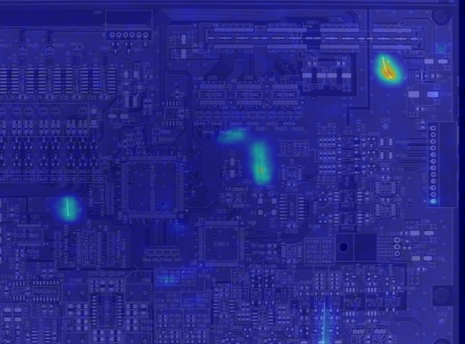
How the score is made. Includes an experiment where you set the threshold yourself on 18 images from a real project.
Read the explainer →
Three-way verdict, processing speed, configuration. The specification table gives the measurement conditions alongside.
See details →
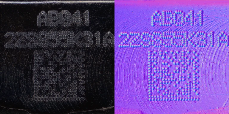
Check, starting from the object, whether the cause of a miss lies in how it is imaged rather than in the decision.
Read the explainer →
Contact
Where to draw the line
is decided by the process.
The loss when a defect is missed, and the effort of a person re-checking one piece. Once these two are known, the operating point can be set. Talk to us, starting with an evaluation run on samples you send us, with the distribution and the confusion matrix shown to you as they come out.