Creating Pseudo-Defects "Just Outside Normal"
 kotai2003
Visual inspection AI in factories is often trained on good parts only, because images of defective parts are hard to collect. So “plausible defects” are created artificially from normal images, and the AI practices telling them apart from normal ones. GLASS, presented at ECCV 2024, reports that it improved the detection of faint and small defects by refining how these pseudo-defects are created.
Conventional pseudo-defects tend to be “questions that are too easy”
There are two main ways to create pseudo-defects. Image-level methods, which paste a different pattern onto the image, look detailed but are limited in variety. Methods that add noise to features (the arrays of numbers obtained by passing an image through a network) are fast. However, the direction cannot be controlled, so some points overlap with normal and others are too far away to be useful practice.
In exam terms, solving only obviously wrong answers will not prepare you for the confusing questions in the real exam. Small scratches and faint stains lie very close to normal in feature space. Unless the boundary separating normal from anomalous is brought close to normal, they will be missed.
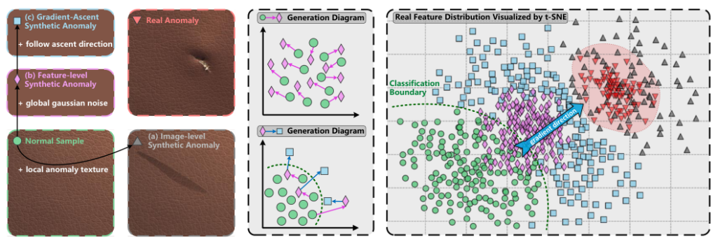
Figure 1 Pseudo-defects from three methods (gray: image-level, pink: Gaussian noise, blue: GLASS). Left: examples on a leather image; center: schematic; right: 2D distribution of features, also showing normal (green) and real defects (red).
Source: Qiyu Chen et al., "A Unified Anomaly Synthesis Strategy with Gradient Ascent for Industrial Anomaly Detection and Localization", ECCV 2024, Fig. 1. https://arxiv.org/abs/2407.09359 (arXiv non-exclusive license; reproduced unmodified as a quotation). The object images in the figure are presumed to come from MVTec AD.
According to the paper, the GLASS pseudo-defects (blue) on the right of Figure 1 cluster near the boundary.
What GLASS changed: two streams of pseudo-defects
GLASS uses two streams of pseudo-defects at the same time. GAS (feature level) covers weak anomalies close to normal, and LAS (image level) covers strong local anomalies far from normal. The discriminator is a small network that outputs an anomaly score from 0 to 1 for each point of the features; it is taught that normal is 0 and pseudo-defects are 1. As shown in Figure 2, the two streams reach the discriminator through separate paths.
flowchart TB
  X["Normal image"] --> F["Feature extractor<br/>+ small adaptor layer"]
  F --> U["Normal features"]
  subgraph GAS["GAS: feature level"]
    direction TB
    G1["Add noise"] --> G2["Move by gradient ascent"] --> G3["Truncated projection"]
  end
  subgraph LAS["LAS: image level"]
    direction TB
    L1["Paste a pattern semi-transparently<br/>with a mottled mask"] --> L2["Same feature extractor"]
  end
  U --> G1
  X --> L1
  U -->|"Normal"| D["Discriminator<br/>anomaly score per point"]
  G3 -->|"Anomalous"| D
  L2 -->|"Pasted area is anomalous"| D
  classDef normal fill:#E8F5E9,stroke:#2E7D32,stroke-width:1px,color:#1B1B1B
  classDef synth fill:#FFF3E0,stroke:#E65100,stroke-width:1px,color:#1B1B1B
  classDef core fill:#FFCC80,stroke:#BF360C,stroke-width:3px,color:#1B1B1B
  classDef judge fill:#E3F2FD,stroke:#1565C0,stroke-width:2px,color:#1B1B1B
  classDef out fill:#EDE7F6,stroke:#4527A0,stroke-width:1px,color:#1B1B1B
  classDef neutral fill:#F5F5F5,stroke:#757575,stroke-width:1px,color:#1B1B1B
  class X,U normal
  class F,L2 neutral
  class G1,L1 synth
  class G2,G3 core
  class D judge
  style GAS fill:#FFF8E1,stroke:#E65100,stroke-width:1px
  style LAS fill:#FFFDE7,stroke:#F9A825,stroke-width:1px
Figure 2 Configuration during training.
LAS cuts out an external texture image with a mottled mask and overlays it with varying transparency, so it can also create faint defects.
Why it works: gradient ascent and truncated projection
GAS first moves the noise-added features, little by little, in the direction that makes it harder for the discriminator to call them “anomalous.” Because the input side is moved in the direction that increases the discriminator’s error, this is called “gradient ascent.” What is moved is not the discriminator’s weights but the features themselves. This produces confusing pseudo-defects.
However, if they are moved too much they overlap with normal, and if they are too far away they are not useful practice either. So every few steps, the distance from the original normal features is measured and kept within a range (a band) between a lower and an upper limit. Features that are too close are pushed out, and features that are too far are pulled back (truncated projection). Figure 3 shows this loop.
flowchart TB
  U["Normal features"] --> N["Noise-added features"]
  N --> A["Move slightly by gradient ascent<br/>toward harder-to-call-anomalous"]
  A -->|"Every few steps"| C{"Truncated projection: distance<br/>from original normal features"}
  C -->|"Below lower limit"| P1["Push out to lower limit"]
  C -->|"Above upper limit"| P2["Pull back to upper limit"]
  C -->|"Within band"| K["Keep as is"]
  P1 & P2 & K --> R{"Reached the set<br/>number of steps?"}
  A -->|"Other steps"| R
  R -->|"Not yet: repeat"| A
  R -->|"Reached"| B["Pseudo-defects within the band<br/>taught as anomalous"]
  classDef normal fill:#E8F5E9,stroke:#2E7D32,stroke-width:1px,color:#1B1B1B
  classDef synth fill:#FFF3E0,stroke:#E65100,stroke-width:1px,color:#1B1B1B
  classDef core fill:#FFCC80,stroke:#BF360C,stroke-width:3px,color:#1B1B1B
  classDef judge fill:#E3F2FD,stroke:#1565C0,stroke-width:2px,color:#1B1B1B
  classDef out fill:#EDE7F6,stroke:#4527A0,stroke-width:1px,color:#1B1B1B
  classDef neutral fill:#F5F5F5,stroke:#757575,stroke-width:1px,color:#1B1B1B
  class U normal
  class N synth
  class A,C,P1,P2 core
  class K,R neutral
  class B synth
Figure 3 Flow of GAS. The direction of movement is kept; only the length is fitted into the band.
At inference, as shown in Figure 4, the inspection image is simply converted into features and passed through the discriminator, which yields a pixel-level anomaly map and an image score.
flowchart LR
  X["Inspection image"] --> F["Feature extractor<br/>+ small adaptor layer"] --> D["Discriminator"] --> Z["Anomaly score per point"]
  Z --> M["Upsample and smooth<br/>pixel anomaly map"]
  Z --> S["Maximum<br/>image anomaly score"]
  classDef normal fill:#E8F5E9,stroke:#2E7D32,stroke-width:1px,color:#1B1B1B
  classDef synth fill:#FFF3E0,stroke:#E65100,stroke-width:1px,color:#1B1B1B
  classDef core fill:#FFCC80,stroke:#BF360C,stroke-width:3px,color:#1B1B1B
  classDef judge fill:#E3F2FD,stroke:#1565C0,stroke-width:2px,color:#1B1B1B
  classDef out fill:#EDE7F6,stroke:#4527A0,stroke-width:1px,color:#1B1B1B
  classDef neutral fill:#F5F5F5,stroke:#757575,stroke-width:1px,color:#1B1B1B
  class X,F neutral
  class D,Z judge
  class M,S out
Figure 4 Flow at inference (no pseudo-defect synthesis).
Results: saturated on standard data, a gap appears on weak defects
AUROC, the metric used here, is the probability that, when one normal and one anomalous image are picked, the anomalous one is scored higher; 100% is perfect. Table 1 compares four evaluation sets. GLASS-m and -h are variants with different distance criteria, and -j selects either m or h for each category.
| Evaluation set (average) | Method | Image AUROC (%) | Pixel AUROC (%) | PRO (%) |
|---|---|---|---|---|
| MVTec AD (15 categories) | GLASS-j | 99.9 | 99.3 | 96.8 |
| Same as above | GLASS-h | 99.8 | 99.0 | 95.9 |
| Same as above | SimpleNet | 99.5 | 98.1 | 90.0 |
| Same as above | BGAD | 97.9 | 98.2 | 96.3 |
| MPDD (6 categories) | GLASS-j | 99.6 | 99.4 | 98.2 |
| Same as above | GLASS-h | 96.7 | 98.8 | 96.4 |
| Same as above | SimpleNet | 98.1 | 98.7 | 95.7 |
| MAD-man (real weak defects selected by people) | GLASS-m | 99.6 | 99.3 | 97.5 |
| Same as above | SimpleNet | 99.3 | 98.6 | 94.8 |
| MAD-sys (synthesized weak defects, created with the same formula as LAS) | GLASS-m | 95.6 | 93.3 | 80.3 |
| Same as above | PatchCore | 92.4 | 92.6 | 63.9 |
| Same as above | SimpleNet | 84.6 | 85.0 | 57.3 |
Table 1 From Tables 2 and 3 of the paper (it is unclear whether the comparison methods were re-run or quoted). PRO measures overlap per defect region, so small defects are counted with the same weight.
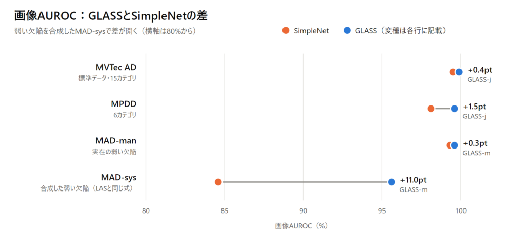
Figure 5 Plotted from the image AUROC in Table 1. Orange: SimpleNet; blue: GLASS (variant shown in each row). The horizontal axis starts at 80%.
SimpleNet, which adds Gaussian noise to features, is the direct point of comparison. Figure 5 shows the difference in image AUROC between the two. On the standard MVTec AD the gap is small, 0.4 points, but on MAD-sys, which contains synthesized faint defects, it widens to 11.0 points. The gap to the runner-up, PatchCore, is 3.2 points. In an ablation that adds components one at a time, image AUROC rose slightly with each addition of gradient ascent and truncated projection.
Limitations and how to read this in practice
- MAD-sys was created with the same formula as LAS, which may favor GLASS. On real weak defects (MAD-man), the gap to SimpleNet in image AUROC is only 0.3 points.
- Not every variant wins: GLASS-h falls below SimpleNet in image AUROC on MPDD.
- The scope is structural anomalies such as scratches and stains; missing or misplaced components were not examined. The method also depends on an external collection of texture images.
If you are considering adoption, the surest approach is probably to collect the faint defects your own line is missing and compare the method side by side with existing ones.
Sources
- Qiyu Chen, Huiyuan Luo, Chengkan Lv, Zhengtao Zhang. "A Unified Anomaly Synthesis Strategy with Gradient Ascent for Industrial Anomaly Detection and Localization." ECCV 2024. https://arxiv.org/abs/2407.09359 (arXiv non-exclusive license)
- The object images in Figure 1 are presumed to come from MVTec AD (https://www.mvtec.com/company/research/datasets/mvtec-ad) (CC BY-NC-SA 4.0, non-commercial). The paper does not state their source.
- Explanatory video: https://youtu.be/ip_WIpqyxr0?si=37nS8xoQWvBiuFot