
A Hands-On Guide to Evaluating AI Anomaly Detection (4/4)
 kotai2003
A tutorial for getting a feel for thresholds, the confusion matrix, and ROC/PR/F1 curves by moving sliders
When companies introduce AI visual inspection, the part most often misunderstood is "evaluation."
You may be told, "We will set the threshold where F1 is highest," but what is F1, why does the threshold change the results,
and how far can you trust a figure like 100%? Discussions often move ahead before these points really sink in.
In this article, you will operate a browser-based learning app as you read, building a hands-on understanding of the evaluation process for anomaly detection
one step at a time. No formulas to memorize. Just move the sliders
and watch the numbers and graphs move together, and you will grasp the overall picture of evaluation.
App (free, no installation required)
https://anomalydetectiondemo.streamlit.app/We recommend opening this article in a separate window and reading it while you operate the app.
All data shown is simulated data for explanation purposes, not data from real products.
What you will learn in this tutorial
- The relationship between the anomaly score and the threshold, and the trade-off between "false detections and missed defects"
- What the confusion matrix and the five evaluation metrics (Recall / Precision / F1 and others) represent
- How to read ROC / PR / F1 curves, and five ways to set the threshold
- An evaluation pitfall: "Even the same AI gets different scores depending on the sample"
Each part includes 🖱 Try it and 👀 Observe steps. Please try them yourself.
Part 4. The luck of the draw: why "sample size" matters
Finally, let's experience an evaluation pitfall. Open "Random numbers" in the left sidebar.
The "seed" is the "lottery ticket number" for the random numbers. It is fixed, so the dots do not move when you change the threshold.
The "Redraw samples" button draws a different set of samples while keeping the distribution settings unchanged.
Think of it as "sampling inspection from the same line again, on a different day."
🖱 Try it 5: redraw with the default (120 good parts, 100 defects)
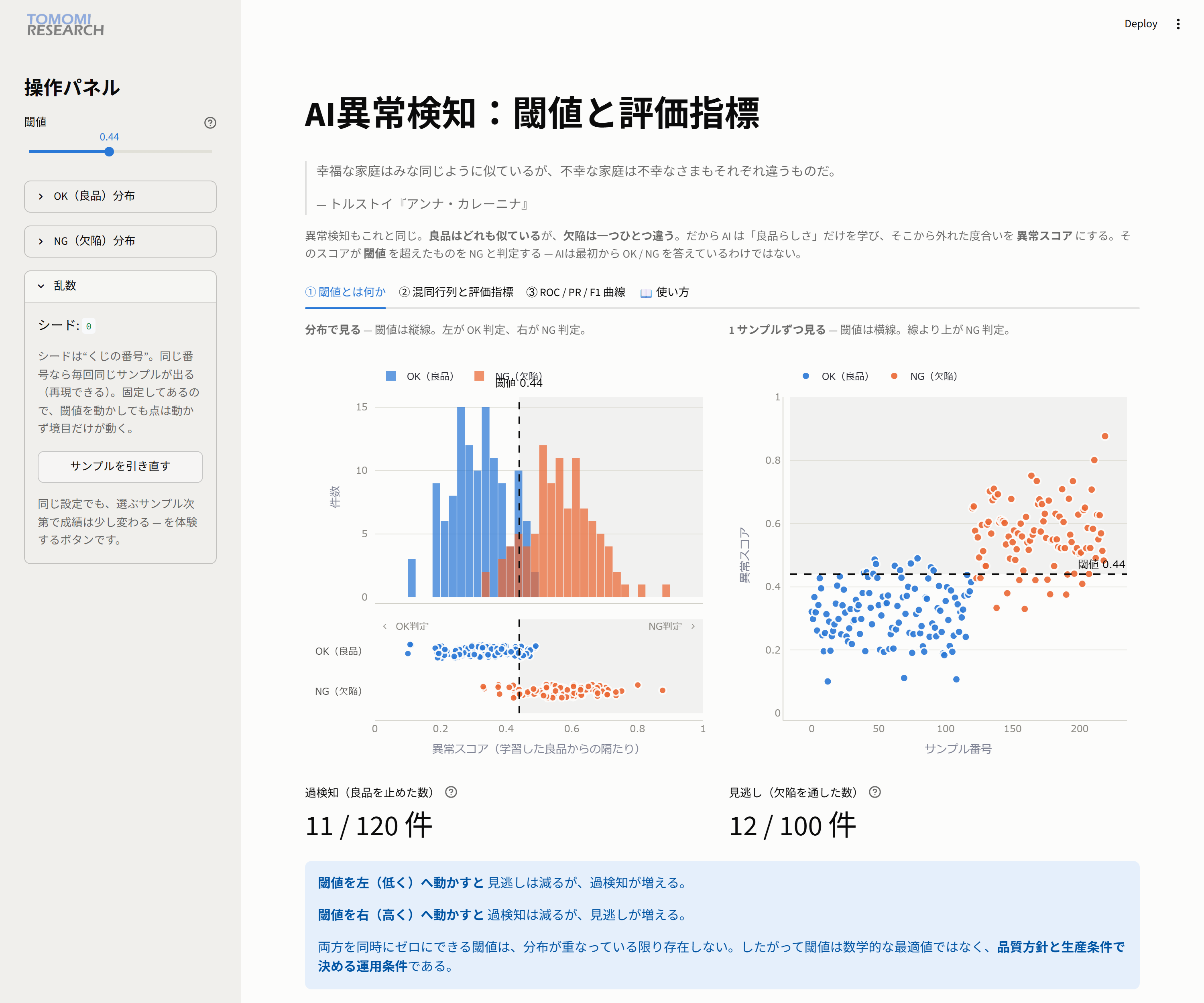
First draw: 11 false detections / 12 missed defects. Press "Redraw samples" once, and...
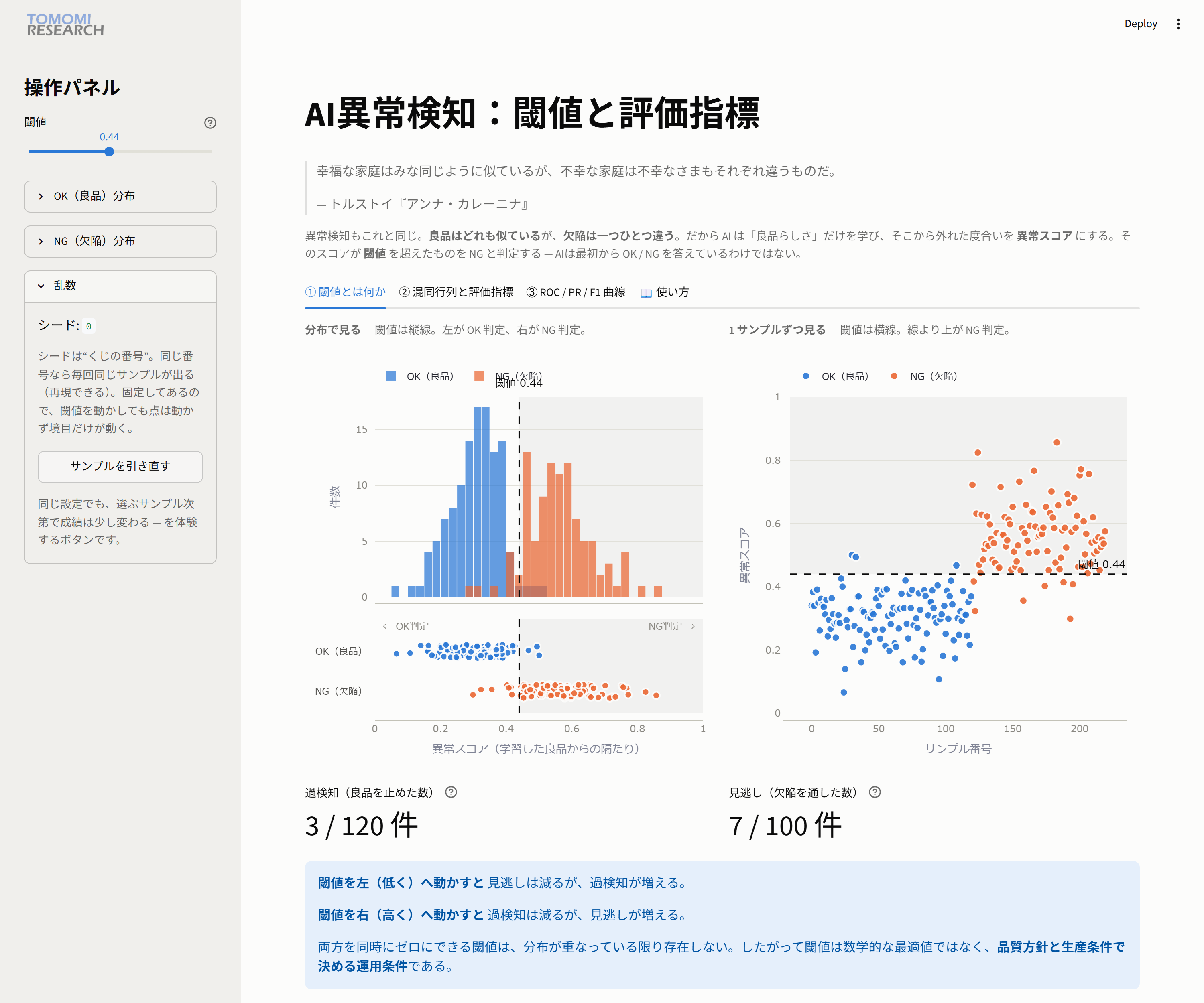
Second draw: 3 false detections / 7 missed defects. The capability of the line (the AI) is the same, yet the numbers changed.
This is the luck of the draw in sampling, which is always part of any evaluation.
🖱 Try it 6: reduce the samples and redraw
In the sidebar, reduce good parts to 15 and defects to 8, then redraw again.
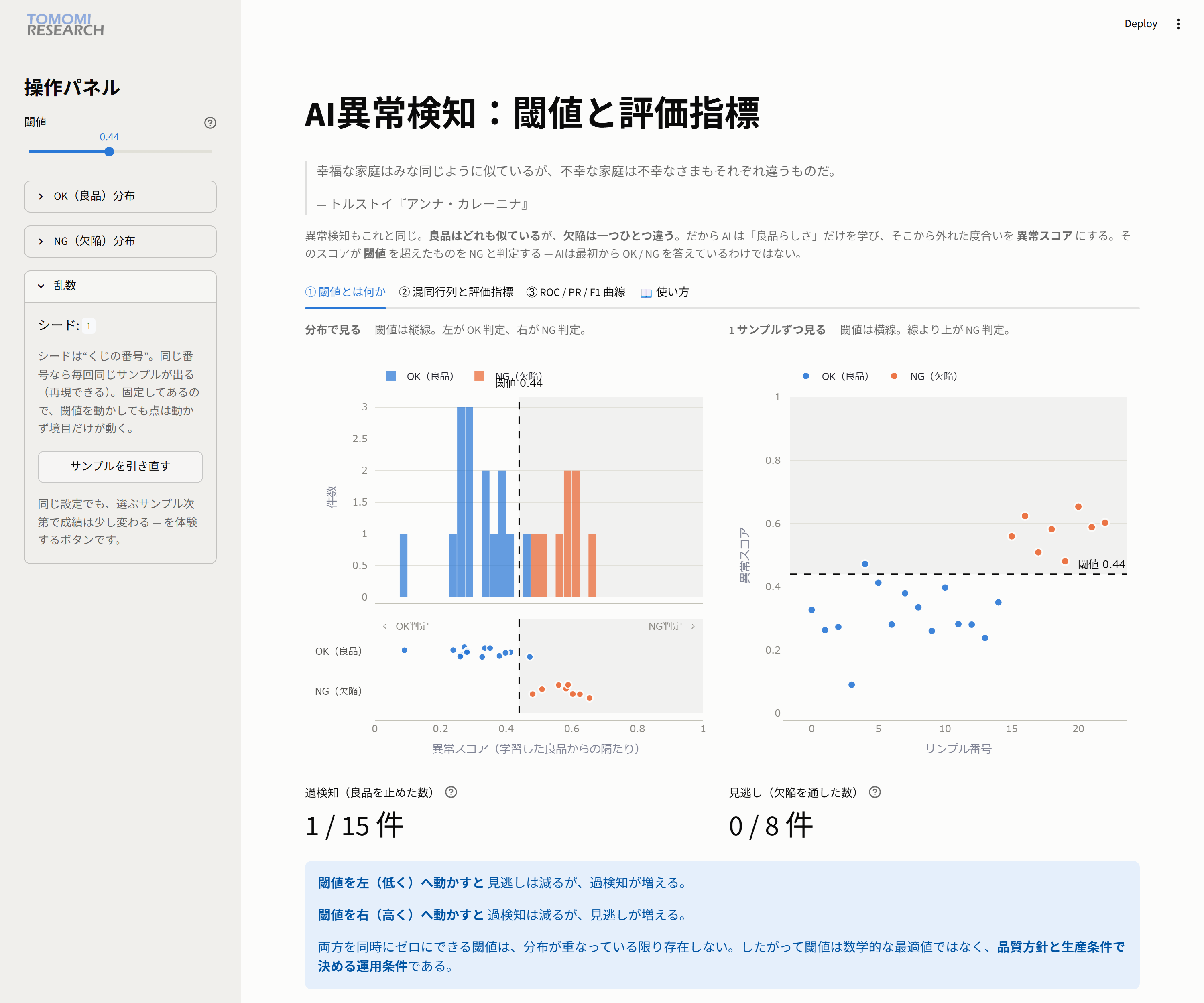
👀 Observe: the histogram has become sparse. False detections 1 / 15, missed defects 0 / 8, Recall 100%.
At first glance this looks "flawless," but it is 100% on only 8 defects.
Redraw once more and false detections change to 2/15. A single judgment moves the metrics by several percent to more than ten percent.
The same Recall of 100% means very different reliability with 8 defects than with 300.
A "100%" obtained from a small sample is no guarantee for mass production.
The purpose of increasing the sample size is not to make the results look better,
but to confirm that the chosen threshold and the evaluation are not "a coincidence."
Summary: the big picture of the anomaly detection evaluation process
Putting the steps you have worked through on a single page, this is what evaluation looks like.
Learn what a good part looks like (training on good parts)
        ↓
Assign an anomaly score to each sample
        ↓
Draw the OK / NG line with the threshold   ← trade-off: false detections ⇄ missed defects
        ↓
Confusion matrix (TP/TN/FP/FN) → Recall / Precision / F1 ...   ← all move together
        ↓
Look at the big picture with ROC / PR / F1, and set the threshold by quality policy
        ↓
(Considering the luck of the draw, evaluate independently with enough samples)
Five things to remember:
- The AI measures "the distance from good parts (the anomaly score)" and separates OK/NG with a threshold.
- False detections and missed defects are a trade-off. Bringing both to zero is impossible (as long as the distributions overlap).
- The confusion matrix and every evaluation metric are calculated from the same four numbers, and they all move together with the threshold.
- AUC is the AI's capability; the threshold is an operational choice. Your quality policy decides the "optimal threshold."
- 100% on a small sample is not a guarantee. Every evaluation includes the luck of the draw.
Please try the app for yourself. When you see everything above move at once
with a single slider, the "map" of evaluation will stick in your mind.
Appendix: quick glossary
| Term | Meaning |
|---|---|
| Anomaly score | A score for the distance from good parts (0 to 1). The larger, the more it looks like a defect |
| Threshold | The boundary beyond which an item is judged NG |
| False detection (FP) | An error that judges a good part NG |
| Missed defect (FN) | An error that judges a defect OK |
| Recall (detection rate) | The share of defects that were detected = TP/(TP+FN) |
| Precision | The share of NG judgments that were actually defects = TP/(TP+FP) |
| F1 Score | The harmonic mean of Recall and Precision |
| ROC / AUC | The performance curve across all thresholds, and the area under it (the capability of the detector) |
| PR curve | The curve showing the relationship between Recall and Precision |

